Commutators

The commutator of two operators $A$ and $B$ is

$$[A,B]=AB-BA.$$

It records how the two possible orderings differ. Acting on a state,

$$[A,B]|\psi\rangle = A(B|\psi\rangle)-B(A|\psi\rangle).$$

The commutator is itself an operator, not a scalar measure of “noncommutativity.” Its action can vanish on one state while remaining nonzero elsewhere, and a scalar size requires an additional choice such as an operator norm or a state-dependent expectation value.

In quantum mechanics, commutators connect several structures:

• $[A,B]=0$ is the finite-dimensional test for compatible sharp observables.
• $[H,A]$ controls how $A$ changes in time.
• $[G,A]$ controls how $A$ transforms under the continuous symmetry generated by $G$.
• $\langle[A,B]\rangle$ enters uncertainty relations.
• Closed commutator relations define Lie algebras such as angular momentum.

This page develops those physical roles and the identities needed to use them. The reusable algebra catalog is Commutators and Anticommutators, and the compact lookup entry is Commutator Identities.

Definition and Ordering Convention

Operator products act from right to left:

$$AB|\psi\rangle = A\left(B|\psi\rangle\right).$$

Therefore $AB$ means “apply $B$, then apply $A$,” whereas $BA$ reverses that order. The commutator is the difference between the resulting vectors.

For matrices or bounded operators, both products are defined on the entire Hilbert space. For unbounded operators, the natural commutator domain is

$$\mathcal D([A,B]) = \mathcal D(AB)\cap\mathcal D(BA),$$

which may be smaller than either individual operator domain. Domain issues are not decoration: without a common domain, the formal difference $AB-BA$ does not define an operator.

If $A$ and $B$ carry physical units, then $[A,B]$ carries the product of those units. For example,

$$[x,p]=i\hbar I$$

has the dimensions of action.

Three Different Vanishing Statements

The following claims are not equivalent:

$$[A,B]=0,$$ $$[A,B]|\psi\rangle=0,$$

and

$$\langle\psi|[A,B]|\psi\rangle=0.$$

The first is an operator identity on the declared space or domain. The second says that the two orderings agree only on one state. The third says only that their difference has zero expectation in that state.

For example,

$$[\sigma_x,\sigma_y]=2i\sigma_z\ne0.$$

Yet in the $\sigma_x$ eigenstate $|+x\rangle$,

$$\langle+x|[\sigma_x,\sigma_y]|+x\rangle = 2i\langle+x|\sigma_z|+x\rangle =0.$$

A vanishing expectation value in one state does not establish compatibility.

Symmetric and Antisymmetric Products

The commutator and anticommutator split an ordered product into antisymmetric and symmetric parts:

$$AB = \frac12\{A,B\} + \frac12[A,B],$$

where

$$\{A,B\}=AB+BA.$$

Reversing the order flips only the commutator term:

$$BA = \frac12\{A,B\} - \frac12[A,B].$$

The symmetric product contributes to covariance, while the antisymmetric product contributes to the commutator part of the uncertainty relation. The separate operator-algebra role of the symmetric bracket is developed in Anticommutators.

Hermiticity Properties

Let $A$ and $B$ be Hermitian matrices or suitably defined self-adjoint operators. Then

$$(AB)^{\dagger}=BA.$$

Consequently, $AB$ is Hermitian exactly when $A$ and $B$ commute, subject to the usual domain qualifications. The commutator satisfies

$$[A,B]^{\dagger} = [B,A] = -[A,B].$$

Thus the commutator of Hermitian operators is anti-Hermitian. Multiplying by $1/i=-i$ produces a Hermitian operator:

$$C_{AB} = \frac1i[A,B].$$

For any state in the relevant domain,

$$\langle[A,B]\rangle^{*} = -\langle[A,B]\rangle,$$

so $\langle[A,B]\rangle$ is purely imaginary. Equivalently,

$$\operatorname{Im}\langle AB\rangle = \frac1{2i} \langle[A,B]\rangle,$$

while

$$\operatorname{Re}\langle AB\rangle = \frac12 \langle\{A,B\}\rangle.$$

These relations explain the factors of $i$ that accompany commutators in equations for real observable quantities.

The Eigenbasis Diagnostic

Suppose $A$ has an orthonormal eigenbasis:

$$A|a_n\rangle=a_n|a_n\rangle.$$

Take a matrix element of the commutator in this basis:

$$\begin{aligned} \langle a_m|[A,B]|a_n\rangle &= \langle a_m|AB-BA|a_n\rangle \\ &= (a_m-a_n) \langle a_m|B|a_n\rangle. \end{aligned}$$

Writing

$$B_{mn}=\langle a_m|B|a_n\rangle,$$

the result is

$$[A,B]_{mn} = (a_m-a_n)B_{mn}.$$

This compact formula contains the simultaneous-diagonalization logic:

• diagonal entries vanish automatically because $a_m-a_m=0$;
• if $a_m\ne a_n$ and $[A,B]=0$, then $B_{mn}=0$;
• $B$ can have nonzero matrix elements only within degenerate eigenspaces of $A$;
• if $A$ is nondegenerate and $[A,B]=0$, then $B$ is diagonal in the $A$-eigenbasis.

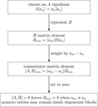
In an $A$ eigenbasis, the commutator weights $B_{mn}$ by $a_m-a_n$. If the commutator vanishes, $B$ cannot connect eigenspaces with different $A$ eigenvalues, although it may still act inside degenerate blocks.

The full projector and measurement interpretation belongs to Compatible Observables.

Core Identities

Commutator identities follow from associativity and distributivity of operator multiplication. They do not require $A$, $B$, and $C$ to be Hermitian.

Bilinearity

For scalars $\alpha$ and $\beta$,

$$[A,\alpha B+\beta C] = \alpha[A,B]+\beta[A,C],$$

and

$$[\alpha A+\beta B,C] = \alpha[A,C]+\beta[B,C].$$

Antisymmetry

$$[A,B]=-[B,A], \qquad [A,A]=0.$$

The identity operator is central:

$$[A,I]=0.$$

Product rules

The commutator acts like a derivative on products:

$$[A,BC] = [A,B]C+B[A,C],$$

and

$$[AB,C] = A[B,C]+[A,C]B.$$

For example,

$$\begin{aligned} [A,BC] &=ABC-BCA \\ &=(ABC-BAC) \\ &\quad+(BAC-BCA) \\ &=[A,B]C+B[A,C]. \end{aligned}$$

The inserted terms $-BAC+BAC$ preserve operator order and make the two commutators visible.

Powers

Repeated use of the product rule gives

$$[A,B^n] = \sum_{r=0}^{n-1} B^r[A,B]B^{n-1-r}.$$

If $[A,B]$ also commutes with $B$, this simplifies to

$$[A,B^n] = n[A,B]B^{n-1}.$$

Without that extra condition, moving $[A,B]$ through the powers of $B$ is not valid.

Jacobi identity

The nested brackets obey

$$[A,[B,C]] + [B,[C,A]] + [C,[A,B]] =0.$$

This identity is what turns an associative operator algebra into a Lie algebra under the commutator bracket.

The broader set of power, inverse, exponential, and mixed commutator identities is kept in the Mathematical Toolkit rather than duplicated here.

Commutator as a Derivation

Define the adjoint action

$$\operatorname{ad}_A(B) = [A,B].$$

The product rule becomes

$$\operatorname{ad}_A(BC) = \operatorname{ad}_A(B)C + B\operatorname{ad}_A(C).$$

Thus $\operatorname{ad}_A$ is a derivation of the operator algebra. The Jacobi identity implies

$$[ \operatorname{ad}_A, \operatorname{ad}_B ](C) = \operatorname{ad}_{[A,B]}(C).$$

In words, the commutator of two infinitesimal adjoint actions is generated by the commutator of their generators. This closure is central to continuous symmetries and Lie algebras.

Commutators and Compatible Observables

For self-adjoint matrices,

$$[A,B]=0$$

is equivalent to simultaneous diagonalizability, commuting spectral projectors, and the existence of a common sharp projective refinement.

If $A$ is degenerate, $B$ need not be diagonal in an arbitrary $A$ eigenbasis. The eigenbasis diagnostic shows exactly what commutation guarantees: $B$ is block diagonal with respect to the distinct eigenspaces of $A$, and it can be diagonalized within each block.

For unbounded self-adjoint operators, a formal commutator that vanishes on a small common domain need not imply compatibility. The robust condition is commutation of the spectral projections, sometimes called strong commutativity.

Noncommutativity and Measurement Order

A nonzero commutator signals that operator order matters somewhere, but $AB$ and $BA$ are not by themselves universal formulas for two sequential measurement probabilities. Actual sequential measurements require spectral projectors and a state-update instrument.

For ideal projective measurements with projectors $P_a$ and $Q_b$, the order dependence appears through products such as

$$Q_bP_a\rho P_aQ_b$$

and

$$P_aQ_b\rho Q_bP_a.$$

If all $P_a$ commute with all $Q_b$, the ideal joint statistics become order independent. Otherwise they can differ. The operational calculation belongs to Sequential Measurements, while the conceptual consequences are developed in Noncommuting Observables.

Commutators and Uncertainty

For observables $A$ and $B$ in a state $|\psi\rangle$, the Robertson relation is

$$\Delta A\,\Delta B \ge \frac12 \left| \langle[A,B]\rangle \right|.$$

The anti-Hermiticity of $[A,B]$ ensures that the expectation value on the right is purely imaginary before its absolute value is taken.

A nonzero operator commutator can nevertheless have zero expectation in a particular state, as the Pauli example above shows. In that state, the simple Robertson lower bound may be zero even though the observables remain incompatible. The stronger Robertson–Schrödinger relation also contains a symmetric covariance term.

The derivation, equality condition, and interpretation are the subject of General Uncertainty Relations.

Commutators Generate Transformations

Let a self-adjoint generator $G$ define the one-parameter unitary family

$$U(\epsilon) = \exp\left( -\frac{i\epsilon G}{\hbar} \right).$$

Using the convention

$$A(\epsilon) = U^{\dagger}(\epsilon)AU(\epsilon),$$

differentiation at $\epsilon=0$ gives

$$\left. \frac{dA(\epsilon)}{d\epsilon} \right|_{\epsilon=0} = \frac{i}{\hbar}[G,A].$$

Therefore

$$A(\epsilon) = A + \frac{i\epsilon}{\hbar}[G,A] + O(\epsilon^2).$$

The sign changes if one uses $UAU^{\dagger}$ instead, so the transformation convention must be stated.

More generally, repeated commutators give the conjugation series

$$\begin{aligned} U^{\dagger}AU &=A + \frac{i\epsilon}{\hbar}[G,A] \\ &\quad+ \frac1{2!} \left( \frac{i\epsilon}{\hbar} \right)^2 [G,[G,A]] +\cdots. \end{aligned}$$

This is the adjoint form of the exponential map. Its detailed symmetry interpretation belongs to Generators, and the exponential algebra belongs to Matrix Functions and Exponentials.

Translation Example

Momentum generates translations. Let

$$U(a)=\exp\left(-\frac{iap}{\hbar}\right).$$

Using

$$[p,x]=-i\hbar I,$$

the first commutator in the conjugation series gives

$$\frac{ia}{\hbar}[p,x]=aI.$$

All higher nested commutators vanish because $[p,I]=0$. Hence

$$U^{\dagger}(a)xU(a) = x+aI.$$

The canonical commutator therefore states not only that $x$ and $p$ are incompatible, but also that momentum shifts the position observable by the translation parameter.

Hamiltonian Commutators and Dynamics

For a time-independent Hamiltonian,

$$U(t)=\exp\left(-\frac{iHt}{\hbar}\right).$$

The Heisenberg-picture operator

$$A_H(t)=U^{\dagger}(t)A_SU(t)$$

satisfies

$$\frac{dA_H}{dt} = \frac{i}{\hbar}[H_H,A_H] + \left( \frac{\partial A}{\partial t} \right)_H.$$

If $A$ has no explicit time dependence and

$$[H,A]=0,$$

then $A_H$ is constant in time. The full dynamical derivation is in Commutator Dynamics, and the expectation-value statement is in Conservation Laws.

Successive Transformations

For matrices $X$ and $Y$ and a small dimensionless parameter $\epsilon$, the group commutator obeys

$$\begin{aligned} &e^{\epsilon X} e^{\epsilon Y} e^{-\epsilon X} e^{-\epsilon Y} \\ &\qquad = I+\epsilon^2[X,Y]+O(\epsilon^3). \end{aligned}$$

The first-order effects cancel. The leading failure of the two transformations to commute is generated by $[X,Y]$. For rotations, this fact is the local algebraic origin of why rotations about different axes do not commute.

Trace and Finite-Dimensional Constraints

For finite matrices, cyclicity of the trace gives

$$\operatorname{Tr}[A,B] = \operatorname{Tr}(AB) - \operatorname{Tr}(BA) =0.$$

The converse is false: most traceless matrices are not zero, and trace zero does not imply that two operators commute.

This identity proves that the canonical commutation relation cannot be represented exactly by finite matrices. If $X$ and $P$ were $d\times d$ matrices satisfying

$$[X,P]=i\hbar I_d,$$

then taking the trace would give

$$0=i\hbar d,$$

which is impossible for $d>0$. Exact canonical pairs therefore require an infinite-dimensional setting, with the associated domain subtleties. Finite matrix truncations can approximate selected matrix elements but cannot obey the exact relation globally.

Example: A Two-Level Matrix

Let

$$A= \begin{pmatrix} a_1&0\\ 0&a_2 \end{pmatrix}, \qquad B= \begin{pmatrix} b_{11}&b_{12}\\ b_{12}^{*}&b_{22} \end{pmatrix}.$$

Then

$$[A,B] = \begin{pmatrix} 0&(a_1-a_2)b_{12}\\ (a_2-a_1)b_{12}^{*}&0 \end{pmatrix}.$$

If $a_1\ne a_2$, the operators commute exactly when

$$b_{12}=0.$$

If $a_1=a_2$, then $A=a_1I$ and commutes with every $B$. This is the simplest example of degeneracy allowing nontrivial action within an $A$ eigenspace.

Example: Pauli Matrices

The Pauli product identity is

$$\sigma_i\sigma_j = \delta_{ij}I + i\sum_k\epsilon_{ijk}\sigma_k.$$

Reversing $i$ and $j$ changes the sign of the antisymmetric term, so

$$[\sigma_i,\sigma_j] = 2i\sum_k\epsilon_{ijk}\sigma_k.$$

In particular,

$$[\sigma_x,\sigma_y]=2i\sigma_z.$$

For spin operators $S_i=(\hbar/2)\sigma_i$, this becomes

$$[S_i,S_j] = i\hbar \sum_k\epsilon_{ijk}S_k.$$

The right-hand side remains inside the span of the spin generators: their commutator algebra closes.

Example: Position and Momentum

On a suitable test function $\psi(x)$, take

$$\begin{aligned} (x\psi)(x) &=x\psi(x), \\ (p\psi)(x) &=-i\hbar\frac{d\psi}{dx}. \end{aligned}$$

Then

$$\begin{aligned} ([x,p]\psi)(x) &=-i\hbar x\psi'(x) \\ &\quad+i\hbar\frac{d}{dx} \left(x\psi(x)\right) \\ &=i\hbar\psi(x). \end{aligned}$$

Thus

$$[x,p]=i\hbar I$$

on the chosen common invariant domain. The multidimensional relations, representation choices, and rigorous qualifications are developed in Canonical Commutation Relations.

Example: Harmonic-Oscillator Ladder Operators

Let

$$[a,a^{\dagger}]=I, \qquad N=a^{\dagger}a.$$

The product rule gives

$$\begin{aligned} [N,a] &=a^{\dagger}[a,a]+[a^{\dagger},a]a \\ &=-a, \end{aligned}$$

and

$$\begin{aligned} [N,a^{\dagger}] &=a^{\dagger}[a,a^{\dagger}] +[a^{\dagger},a^{\dagger}]a \\ &=a^{\dagger}. \end{aligned}$$

If $N|n\rangle=n|n\rangle$, then

$$N(a^{\dagger}|n\rangle) = (n+1)a^{\dagger}|n\rangle,$$

and

$$N(a|n\rangle) = (n-1)a|n\rangle.$$

The commutators reveal the raising and lowering action without first writing wavefunctions. The full construction belongs to Ladder-Operator Solution: First Encounter.

Example: Angular Momentum

Angular momentum satisfies

$$[J_i,J_j] = i\hbar \sum_k\epsilon_{ijk}J_k.$$

These relations express both incompatibility of distinct components and the Lie algebra of rotations. The Casimir operator

$$J^2=J_x^2+J_y^2+J_z^2$$

commutes with every component:

$$[J^2,J_i]=0.$$

The derivation and representation theory are developed in Angular Momentum Algebra.

Classical Poisson-Bracket Correspondence

Canonical quantization motivates the schematic correspondence

$$\frac1{i\hbar}[A,B] \longleftrightarrow \{a,b\}_{\mathrm{PB}}.$$

Both brackets are antisymmetric, satisfy a product rule, and obey the Jacobi identity. This resemblance explains why commutators govern quantum Hamiltonian evolution.

The correspondence is not an exact substitution rule for arbitrary observables. Operator ordering, domain questions, and higher-order quantum corrections obstruct a universal bracket-preserving quantization map. The classical bracket and its geometric meaning belong to Poisson Brackets.

Domain and Strong-Commutation Caveats

For unbounded operators,

$$\mathcal D(AB) = \left\lbrace |\psi\rangle\in\mathcal D(B): B|\psi\rangle\in\mathcal D(A) \right\rbrace,$$

and $\mathcal D(BA)$ is generally different. Symbolic manipulation is safest on a declared dense subspace preserved by all operators in the calculation.

Even if

$$[A,B]|\psi\rangle=0$$

throughout a common dense domain, the spectral projectors of two unbounded self-adjoint operators need not commute. Measurement compatibility requires the stronger spectral statement. Conversely, a commutator formula such as $[x,p]=i\hbar I$ should be read together with the domain on which it is verified.

When domains matter, state them, check that each intermediate vector remains in the next operator’s domain, and distinguish a formal identity from an identity of self-adjoint operators.

A Practical Calculation Workflow

1. Preserve operator order from the start; do not rearrange factors unless a commutation relation justifies it.
2. For unbounded operators, declare a common invariant domain before expanding products.
3. Use bilinearity to separate sums and scalar factors.
4. Use the product rule to reduce composite operators to known basic commutators.
5. Exploit central commutators early; if $[A,B]$ is proportional to $I$, nested commutators often terminate.
6. Check dimensions and Hermiticity. For Hermitian $A$ and $B$, $[A,B]$ must be anti-Hermitian.
7. Distinguish an operator identity from its action or expectation in one state.
8. Test the result in a convenient representation when possible.

Common Mistakes

• Treating $AB$ and $BA$ as interchangeable because ordinary numbers commute.
• Reading $[A,B]$ as a scalar “amount” without choosing a norm or state.
• Concluding $[A,B]=0$ from one vanishing expectation value.
• Assuming noncommuting operators cannot share any eigenvector; they may share some without possessing a complete common basis.
• Treating $AB$ as the universal probability rule for measuring $B$ then $A$.
• Forgetting that the commutator of Hermitian operators is anti-Hermitian.
• Dropping the factors of $i$ or $\hbar$ in generator and dynamics formulas.
• Using $[A,B^n]=n[A,B]B^{n-1}$ without checking that $[A,B]$ commutes with $B$.
• Assuming $e^{A+B}=e^Ae^B$ when $[A,B]\ne0$.
• Ignoring domains for position, momentum, Hamiltonians, and other unbounded operators.
• Seeking exact finite matrices satisfying $[X,P]=i\hbar I$.

Canonical Boundaries

This page owns the physical interpretation and central uses of the commutator. Nearby pages own specialized developments:

• Commutators and Anticommutators owns the reusable finite-dimensional algebra and longer identity list.
• Compatible Observables owns simultaneous diagonalization and common projective refinements.
• Noncommuting Observables owns the measurement and interpretive consequences of noncommutativity.
• Generators owns one-parameter unitary groups and symmetry transformations.
• Commutator Dynamics owns Heisenberg evolution, nested commutators, and dynamical examples.
• General Uncertainty Relations owns the Cauchy–Schwarz derivation and equality conditions.

Summary

• The commutator $[A,B]=AB-BA$ is the operator difference between two orderings.
• Operator vanishing, vanishing on one state, and a vanishing expectation value are different statements.
• For Hermitian $A$ and $B$, the commutator is anti-Hermitian and its expectation value is purely imaginary.
• In an $A$ eigenbasis, $[A,B]_{mn}=(a_m-a_n)B_{mn}$, so commutation means that $B$ preserves eigenspaces of $A$.
• Product rules make $\operatorname{ad}_A(B)=[A,B]$ a derivation, while the Jacobi identity gives a Lie bracket.
• Commutators test sharp-observable compatibility and enter uncertainty bounds, but sequential measurement probabilities require projectors and instruments.
• Commutators with generators control infinitesimal transformations; commutators with the Hamiltonian control time evolution.
• The trace of every finite matrix commutator vanishes, forbidding exact finite-dimensional canonical commutation relations.
• Unbounded operators require explicit domain control, and a formal vanishing commutator is weaker than strong spectral commutativity.

References

• P. A. M. Dirac, The Principles of Quantum Mechanics, 4th ed., Oxford University Press, 1958.
• J. von Neumann, Mathematical Foundations of Quantum Mechanics, Princeton University Press, 1955.
• A. Messiah, Quantum Mechanics, Dover, 1999.
• R. Shankar, Principles of Quantum Mechanics, 2nd ed., Springer, 1994.
• J. J. Sakurai and J. Napolitano, Modern Quantum Mechanics, 3rd ed., Cambridge University Press, 2020.
• C. Cohen-Tannoudji, B. Diu, and F. Laloë, Quantum Mechanics, Wiley, 1977.
• B. C. Hall, Quantum Theory for Mathematicians, Springer, 2013.
• M. Reed and B. Simon, Methods of Modern Mathematical Physics, Vol. I: Functional Analysis, rev. ed., Academic Press, 1980.

Exercises

Exercise 1: Product and power rules

Prove the product rule

$$[A,BC]=[A,B]C+B[A,C],$$

then use it to prove by induction that

$$[A,B^n] = \sum_{r=0}^{n-1} B^r[A,B]B^{n-1-r}.$$

Solution

Insert and subtract $BAC$:

$$\begin{aligned} [A,BC] &=ABC-BCA \\ &=(ABC-BAC) \\ &\quad+(BAC-BCA) \\ &=[A,B]C+B[A,C]. \end{aligned}$$

The power formula is true for $n=1$. Assume it holds for $n$. Then

$$\begin{aligned} [A,B^{n+1}] &=[A,B^n]B+B^n[A,B] \\ &=\sum_{r=0}^{n-1} B^r[A,B]B^{n-r} \\ &\quad+B^n[A,B] \\ &=\sum_{r=0}^{n} B^r[A,B]B^{n-r}. \end{aligned}$$

This is the required formula with $n$ replaced by $n+1$.

Exercise 2: Hermiticity and expectations

Let $A$ and $B$ be Hermitian matrices. Prove that $[A,B]$ is anti-Hermitian and that $\langle[A,B]\rangle$ is purely imaginary in every state.

Solution

Taking the adjoint reverses product order:

$$\begin{aligned} [A,B]^{\dagger} &=(AB-BA)^{\dagger} \\ &=BA-AB \\ &=-[A,B]. \end{aligned}$$

For any normalized $|\psi\rangle$,

$$\begin{aligned} \langle[A,B]\rangle^{*} &=\langle\psi|[A,B]^{\dagger}|\psi\rangle \\ &=-\langle\psi|[A,B]|\psi\rangle. \end{aligned}$$

A complex number $z$ satisfying $z^{*}=-z$ is purely imaginary.

Exercise 3: Eigenbasis block structure

Let $A|a_n\rangle=a_n|a_n\rangle$. Derive

$$\langle a_m|[A,B]|a_n\rangle = (a_m-a_n)B_{mn}.$$

What does $[A,B]=0$ imply when $A$ is nondegenerate? What changes when $A$ is degenerate?

Solution

Using the eigenvalue equations on the bra and ket sides,

$$\begin{aligned} \langle a_m|AB|a_n\rangle &=a_mB_{mn}, \\ \langle a_m|BA|a_n\rangle &=a_nB_{mn}. \end{aligned}$$

Subtracting gives the stated result. If $[A,B]=0$ and $a_m\ne a_n$, then $B_{mn}=0$. For a nondegenerate $A$, every off-diagonal matrix element of $B$ vanishes, so $B$ is diagonal in the $A$ eigenbasis.

If $A$ is degenerate, matrix elements of $B$ may remain nonzero between states with the same eigenvalue. Thus $B$ is block diagonal and may be diagonalized inside each degenerate block.

Exercise 4: A zero commutator expectation

Use $[\sigma_x,\sigma_y]=2i\sigma_z$ to show that the commutator expectation vanishes in $|+x\rangle$, even though the operators do not commute.

Solution

The $|+x\rangle$ state has Bloch vector along the $x$ direction, so

$$\langle+x|\sigma_z|+x\rangle=0.$$

Therefore

$$\begin{aligned} \langle+x|[\sigma_x,\sigma_y]|+x\rangle &=2i\langle+x|\sigma_z|+x\rangle \\ &=0. \end{aligned}$$

But $[\sigma_x,\sigma_y]=2i\sigma_z$ is a nonzero operator. A state-specific expectation cannot replace the operator test.

Exercise 5: Momentum generates translations

Let

$$U(a)=e^{-iap/\hbar}$$

and assume $[x,p]=i\hbar I$. Use the conjugation series to compute $U^{\dagger}(a)xU(a)$.

Solution

The first correction is

$$\frac{ia}{\hbar}[p,x] = \frac{ia}{\hbar}(-i\hbar I) =aI.$$

The next nested commutator vanishes:

$$[p,[p,x]] = -i\hbar[p,I] =0.$$

All later terms also vanish, so

$$U^{\dagger}(a)xU(a)=x+aI.$$

Exercise 6: Number-operator commutators

Given

$$[a,a^{\dagger}]=I, \qquad N=a^{\dagger}a,$$

derive $[N,a]=-a$ and $[N,a^{\dagger}]=a^{\dagger}$. Then show that $a^{\dagger}|n\rangle$ has number eigenvalue $n+1$ whenever it is nonzero.

Solution

Using the product rule,

$$\begin{aligned} [N,a] &=a^{\dagger}[a,a]+[a^{\dagger},a]a \\ &=-a, \end{aligned}$$

and

$$\begin{aligned} [N,a^{\dagger}] &=a^{\dagger}[a,a^{\dagger}] +[a^{\dagger},a^{\dagger}]a \\ &=a^{\dagger}. \end{aligned}$$

Since $[N,a^{\dagger}]=a^{\dagger}$,

$$\begin{aligned} N a^{\dagger}|n\rangle &=(a^{\dagger}N+[N,a^{\dagger}])|n\rangle \\ &=(n+1)a^{\dagger}|n\rangle. \end{aligned}$$

Exercise 7: No finite canonical pair

Prove that no finite-dimensional matrices $X$ and $P$ can satisfy

$$[X,P]=i\hbar I.$$

Solution

For finite matrices,

$$\operatorname{Tr}[X,P] = \operatorname{Tr}(XP)-\operatorname{Tr}(PX) =0$$

by cyclicity. If the canonical relation held in dimension $d$, the same trace would be

$$\operatorname{Tr}(i\hbar I_d) =i\hbar d,$$

which is nonzero for $d>0$. This contradiction rules out an exact finite matrix representation.

Exercise 8: The group commutator

For finite matrices $X$ and $Y$, expand

$$e^{\epsilon X} e^{\epsilon Y} e^{-\epsilon X} e^{-\epsilon Y}$$

through order $\epsilon^2$ and show that the result is

$$I+\epsilon^2[X,Y]+O(\epsilon^3).$$

Solution

Use

$$e^{\pm\epsilon X} = I\pm\epsilon X + \frac{\epsilon^2}{2}X^2 +O(\epsilon^3),$$

and the analogous expansion for $Y$. Multiplying in the written order while preserving every factor gives cancellation of all first-order terms. The second-order terms combine as

$$XY-YX=[X,Y].$$

Let $C_+=e^{\epsilon X}e^{\epsilon Y}$ and $C_-=e^{-\epsilon X}e^{-\epsilon Y}$. Therefore

$$C_+C_- = I+\epsilon^2[X,Y]+O(\epsilon^3).$$