Canonical Commutation Relations

For one canonical coordinate $X$ and its conjugate momentum $P$, the canonical commutation relation is

$$[X,P]=i\hbar I.$$

For $n$ Cartesian degrees of freedom, the canonical algebra is

$$[X_i,P_j]=i\hbar\delta_{ij}I,$$ $$[X_i,X_j]=0, \qquad [P_i,P_j]=0.$$

These are operator relations, not numerical measurement outcomes. They state that each $P_i$ is conjugate to $X_i$, while distinct Cartesian canonical pairs commute in the standard unconstrained theory.

The algebra has several inseparable meanings:

• $X$ and $P$ are incompatible sharp observables.
• $P$ generates translations of $X$.
• $X$ generates translations of $P$.
• position- and momentum-space wavefunctions are Fourier transforms.
• the uncertainty bound $\Delta X\,\Delta P\ge\hbar/2$ follows.
• commutators with functions of $X$ and $P$ reproduce the canonical structure of Hamiltonian dynamics.

The compact equation hides important qualifications. $X$ and $P$ are unbounded, so the raw commutator holds on a suitable common invariant domain, not as an everywhere-defined bounded-operator identity. Its exponentiated Weyl form is often the cleaner rigorous statement.

The bounded Weyl-system owner, including the fixed central phase, regularity, irreducibility boundary, and generator recovery, is Weyl Form of the Canonical Commutation Relations. This Core page retains the physical commutator and uncertainty role.

Why the Pair Is Called Canonical

In classical Hamiltonian mechanics, canonical phase-space coordinates satisfy

$$\{q_i,p_j\}_{\mathrm{PB}}=\delta_{ij},$$ $$\{q_i,q_j\}_{\mathrm{PB}}=0, \qquad \{p_i,p_j\}_{\mathrm{PB}}=0.$$

Canonical quantization replaces these basic brackets schematically by

$$\{\,\cdot\,,\,\cdot\,\}_{\mathrm{PB}} \longrightarrow \frac1{i\hbar} [\,\cdot\,,\,\cdot\,].$$

Applying this rule to the basic coordinates gives the canonical commutation relations. The correspondence is structurally valuable but is not a universal quantization algorithm: nonlinear observables introduce ordering ambiguities, and no prescription preserves every classical Poisson bracket exactly.

The classical geometry belongs to Poisson Brackets, while the distinction between constructing a quantum model and taking a classical limit is developed in Quantization vs Classical Limit.

Schrödinger Representation on the Line

Take

$$\mathcal H=L^2(\mathbb R,dx).$$

On a sufficiently regular wavefunction $\psi$, position acts by multiplication and momentum by differentiation:

$$\begin{aligned} (X\psi)(x) &=x\psi(x), \\ (P\psi)(x) &=-i\hbar\frac{d\psi}{dx}. \end{aligned}$$

The two orderings act as

$$(XP\psi)(x) = -i\hbar x\psi'(x),$$

and

$$\begin{aligned} (PX\psi)(x) &=-i\hbar \frac{d}{dx} \left(x\psi(x)\right) \\ &=-i\hbar\psi(x) -i\hbar x\psi'(x). \end{aligned}$$

Subtracting gives

$$([X,P]\psi)(x) = i\hbar\psi(x).$$

Thus

$$[X,P]=i\hbar I$$

on the chosen common domain. The identity operator is often suppressed in informal notation, but it matters when comparing operator types, taking traces, or generalizing the algebra.

Momentum Representation

Choose the Fourier convention

$$\widetilde\psi(p) = \frac1{\sqrt{2\pi\hbar}} \int_{-\infty}^{\infty} e^{-ipx/\hbar} \psi(x)\,dx.$$

In momentum space,

$$\begin{aligned} (P\widetilde\psi)(p) &=p\widetilde\psi(p), \\ (X\widetilde\psi)(p) &=i\hbar\frac{d\widetilde\psi}{dp}. \end{aligned}$$

Direct calculation again yields

$$[X,P]\widetilde\psi = i\hbar\widetilde\psi.$$

The sign of the derivative representation tracks the sign chosen in the Fourier kernel. A different convention is equally valid if every transform, inverse transform, and translation phase is changed consistently. See Fourier-Transform Conventions and Position and Momentum Representations.

Several Degrees of Freedom

On

$$\mathcal H=L^2(\mathbb R^n,d^nx),$$

the Cartesian Schrödinger representation is

$$\begin{aligned} (X_i\psi)(\mathbf x) &=x_i\psi(\mathbf x), \\ (P_j\psi)(\mathbf x) &=-i\hbar \frac{\partial\psi}{\partial x_j}. \end{aligned}$$

The product rule gives

$$([X_i,P_j]\psi)(\mathbf x) = i\hbar\delta_{ij}\psi(\mathbf x).$$

Thus

$$[X_i,P_j]=i\hbar\delta_{ij}I.$$

When $i\ne j$, differentiating with respect to $x_j$ does not act on the factor $x_i$, so the commutator vanishes.

For many distinguishable particles, add a particle label $\alpha$:

$$[X_{\alpha i},P_{\beta j}] = i\hbar \delta_{\alpha\beta} \delta_{ij}I.$$

Canonical variables belonging to different particle labels or different Cartesian directions commute in this representation.

Symplectic Matrix Form

Collect all canonical operators into

$$Z = (X_1,\ldots,X_n,P_1,\ldots,P_n)^{\mathsf T}.$$

Then the full algebra can be written compactly as

$$[Z_a,Z_b] = i\hbar\Omega_{ab}I,$$

where

$$\Omega = \begin{pmatrix} 0&I_n\\ -I_n&0 \end{pmatrix}.$$

The antisymmetric matrix $\Omega$ is the standard symplectic form in canonical coordinates. Linear transformations $Z\mapsto SZ$ preserve the canonical commutation relations exactly when

$$S\Omega S^{\mathsf T}=\Omega.$$

This matrix form becomes especially useful for coupled oscillators, Gaussian states, and phase-space methods.

Commutators with Powers and Functions

The basic canonical relation and the commutator product rule imply

$$[X,P^n] = i\hbar nP^{n-1},$$

and

$$[P,X^n] = -i\hbar nX^{n-1}.$$

For sufficiently regular functions defined by convergent functional calculus, these become the formal derivative rules

$$[X,f(P)] = i\hbar f'(P),$$

and

$$[P,g(X)] = -i\hbar g'(X).$$

The formulas are exact for polynomials on a common invariant domain. For more general functions and unbounded operators, the domains and functional calculus must be controlled.

Momentum Generates Position Translations

Define the unitary translation operator

$$T(a) = \exp\left(-\frac{iaP}{\hbar}\right).$$

In the position representation,

$$(T(a)\psi)(x)=\psi(x-a).$$

Conjugating $X$ gives

$$T^{\dagger}(a)XT(a) = X+aI.$$

The result follows from the nested-commutator series. The first correction is

$$\frac{ia}{\hbar}[P,X]=aI,$$

and every higher nested commutator vanishes because $[P,I]=0$.

This is the operational generator meaning of the canonical relation: momentum is the infinitesimal generator of spatial translations. The symmetry-side development is Translations and Momentum.

Position Generates Momentum Translations

Define the modulation or momentum-translation operator

$$M(b) = \exp\left(\frac{ibX}{\hbar}\right).$$

It acts in position space as

$$(M(b)\psi)(x) = e^{ibx/\hbar}\psi(x),$$

and shifts momentum under conjugation:

$$M^{\dagger}(b)PM(b) = P+bI.$$

Thus $X$ and $P$ generate translations along the two conjugate directions of phase space.

Weyl Form of the Canonical Relations

The two unitary shifts do not commute. Acting on a wavefunction shows

$$T(a)M(b) = e^{-iab/\hbar} M(b)T(a).$$

The mismatch is a phase in the center of the operator algebra. This is the Weyl relation, the exponentiated form of the canonical commutation relation.

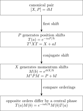
The bracket $[X,P]=i\hbar I$ makes $P$ the generator of position shifts and $X$ the generator of momentum shifts. Performing the shifts in opposite orders changes the state vector by the central phase $e^{-iab/\hbar}$.

Unlike $X$ and $P$, the operators $T(a)$ and $M(b)$ are bounded and defined on the whole Hilbert space. Strongly continuous unitary families also recover self-adjoint generators through Stone’s theorem. For these reasons the Weyl form is often preferable in rigorous representation theory.

The group structure behind the phase is developed in Heisenberg Group.

Stone–von Neumann Uniqueness

For finitely many canonical degrees of freedom, every irreducible, strongly continuous representation of the Weyl relations with the same nonzero central parameter $\hbar$ is unitarily equivalent to the Schrödinger representation.

This result explains why position space and momentum space are two representations of one ordinary canonical quantum theory rather than distinct theories. The Fourier transform supplies the unitary map between them.

The hypotheses are essential:

• the number of degrees of freedom is finite;
• the representation is irreducible;
• the Weyl operators depend strongly continuously on their parameters;
• the central phase is fixed.

With infinitely many degrees of freedom, as in quantum field theory or thermodynamic limits, unitarily inequivalent representations can occur. The exact hypotheses, conclusion, proof architecture, and failure modes belong to the canonical Stone–von Neumann Theorem. The formalism card is its compact lookup projection.

No Exact Finite-Dimensional Canonical Pair

No finite matrices $X$ and $P$ can satisfy

$$[X,P]=i\hbar I.$$

For $d\times d$ matrices, cyclicity gives

$$\operatorname{Tr}[X,P]=0,$$

whereas

$$\operatorname{Tr}(i\hbar I_d) = i\hbar d\ne0.$$

This contradiction is one reason an exact canonical coordinate requires an infinite-dimensional Hilbert space. Finite truncations used in numerics can approximate low-energy matrix elements but must violate the canonical relation somewhere, often near the truncation boundary.

Position–Momentum Uncertainty

The Robertson inequality gives

$$\Delta X\,\Delta P \ge \frac12 \left| \langle[X,P]\rangle \right|.$$

Using the canonical relation,

$$\Delta X\,\Delta P \ge \frac{\hbar}{2}.$$

The bound concerns standard deviations in one prepared state. It is not a claim about finite instrument resolution, and it does not say that either observable lacks a sharp eigenvalue in every generalized sense. The variance derivation, Gaussian equality states, and Fourier interpretation belong to Position–Momentum Uncertainty.

Recovering Hamiltonian Equations

For

$$H=\frac{P^2}{2m}+V(X),$$

the canonical derivative identities give

$$[X,H] = i\hbar\frac{P}{m},$$

and

$$[P,H] = -i\hbar V'(X).$$

The Heisenberg equations therefore read

$$\frac{dX_H}{dt} = \frac{P_H}{m},$$

and

$$\frac{dP_H}{dt} = -V'(X_H).$$

These are operator versions of the classical canonical equations. They do not make the full quantum dynamics classical: $X_H$ and $P_H$ remain operators, states can spread and interfere, and nonlinear expectation values need not close on the expectations alone. The dynamics-side treatment is Commutator Dynamics.

Canonical and Kinetic Momentum in a Magnetic Field

For a particle of charge $q$ in a vector potential $\mathbf A(\mathbf X)$, the canonical momentum in the Cartesian Schrödinger representation is

$$\mathbf P=-i\hbar\boldsymbol\nabla.$$

The kinetic, or mechanical, momentum is

$$\boldsymbol\Pi = \mathbf P-q\mathbf A(\mathbf X).$$

Both satisfy

$$[X_i,P_j] = [X_i,\Pi_j] = i\hbar\delta_{ij}I,$$

because functions of position commute with position. Their component commutators differ:

$$[P_i,P_j]=0,$$

but

$$[\Pi_i,\Pi_j] = iq\hbar \sum_k\epsilon_{ijk}B_k(\mathbf X).$$

The kinetic momentum is proportional to velocity and is gauge covariant; canonical momentum is the variable conjugate to position and the generator appearing in the canonical algebra. Conflating the two hides the magnetic field in precisely the commutator where it has physical consequences.

Domains Are Part of the Relation

On $L^2(\mathbb R)$, a natural position-operator domain is

$$\mathcal D(X) = \left\lbrace \psi\in L^2(\mathbb R): x\psi\in L^2(\mathbb R) \right\rbrace.$$

Momentum is defined on an appropriate Sobolev domain of square-integrable functions with square-integrable weak derivative. The Schwartz space

$$\mathcal S(\mathbb R)$$

is a convenient dense common invariant core: multiplication by $x$ and differentiation both preserve it, and the calculation

$$[X,P]\psi=i\hbar\psi$$

is valid there.

The raw identity does not mean that $XP$, $PX$, and $I$ are bounded operators defined on every vector in $L^2(\mathbb R)$. Boundary conditions also matter. On a finite interval or compact configuration space, self-adjoint momentum operators depend on boundary data, and global canonical coordinates may require a different formulation.

The general operator-domain framework is developed in Unbounded Operators.

Situations Requiring Modification

Periodic coordinates

An angular coordinate is periodic, while angular momentum has a discrete spectrum. A globally defined self-adjoint angle operator cannot satisfy the naive relation

$$[\Phi,L_z]=i\hbar I$$

on all angular-momentum eigenstates. Unitary phase operators such as $e^{i\Phi}$ and their Weyl-type relations are safer global objects.

Energy and time

Ordinary nonrelativistic quantum mechanics treats time as an external parameter, not automatically as a self-adjoint operator $T$ satisfying $[T,H]=i\hbar I$. Energy–time uncertainty therefore requires a different analysis from the position–momentum pair; see Energy–Time Uncertainty.

Constraints and curved coordinates

Constrained systems may require reduced phase-space variables or Dirac brackets before quantization. In curvilinear coordinates, the inner-product measure and self-adjointness can add terms to naive differential momentum operators. The Cartesian formula $P_j=-i\hbar\partial_j$ should not be copied unchanged into every coordinate system.

Quantum fields

For a canonical field and its conjugate momentum, the discrete index becomes a spatial point, schematically giving an equal-time relation

$$[\Phi(t,\mathbf x),\Pi(t,\mathbf y)] = i\hbar\delta^{(d)}(\mathbf x-\mathbf y)I.$$

This is an operator-valued-distribution statement, not an ordinary operator identity at one point. The field-theory construction and constraint caveats belong to From Phase Space to Canonical Quantization.

Physical Interpretation

The canonical commutation relations should be read as one coherent package:

1. Algebra: conjugate operators fail to commute by a central amount set by $\hbar$.
2. Geometry: the commutator is the quantum image of the symplectic form on phase space.
3. Transformations: each canonical operator generates translations of its conjugate.
4. Representations: position and momentum descriptions are related by a unitary Fourier transform.
5. Probabilities: no state with finite variances can make both spreads arbitrarily small.
6. Dynamics: canonical commutators turn Hamiltonians into equations of motion through Heisenberg evolution.

No single slogan such as “measurement disturbs the system” captures all of this structure.

Sign and Convention Checks

With

$$P=-i\hbar\frac{d}{dx},$$

the canonical sign is

$$[X,P]=+i\hbar I, \qquad [P,X]=-i\hbar I.$$

With

$$T(a)=e^{-iaP/\hbar}, \qquad M(b)=e^{ibX/\hbar},$$

the Weyl phase is

$$T(a)M(b) = e^{-iab/\hbar}M(b)T(a).$$

Changing the Fourier kernel or choosing the opposite active/passive translation convention changes several signs together. A reliable check is to act on a test wavefunction and verify both the shift direction and the commutator.

A Practical Audit

When using canonical commutation relations:

1. Identify the actual canonical variables and distinguish them from kinetic or constrained variables.
2. State the Hilbert space, representation, and Fourier convention.
3. Preserve the identity operator when the operator type matters.
4. For differential operators, specify a common invariant domain or core.
5. Use the product rule to derive composite commutators instead of treating operators as ordinary numbers.
6. Check dimensions: $[Q,P]$ must have units of action.
7. For global or rigorous statements, prefer the exponentiated Weyl relation.
8. Do not assume finite truncations, compact coordinates, or field operators obey the naive Cartesian relation without modification.

Common Mistakes

• Writing $[X,P]=i\hbar$ as though the right-hand side were a scalar rather than $i\hbar I$.
• Reversing the sign between $[X,P]$ and $[P,X]$.
• Forgetting the Kronecker delta in several dimensions.
• Calling kinetic momentum and canonical momentum the same object in a magnetic field.
• Treating the commutator as a measured value rather than an operator relation.
• Assuming the raw unbounded commutator holds on every Hilbert-space vector.
• Claiming that finite matrices can realize the exact canonical relation.
• Applying the Stone–von Neumann theorem to infinitely many degrees of freedom.
• Treating time as automatically another position operator conjugate to the Hamiltonian.
• Copying $-i\hbar\partial_q$ into curvilinear or constrained coordinates without checking the measure and self-adjoint domain.
• Using the Poisson-bracket replacement as a universal quantization algorithm.

Canonical Boundaries

This page owns the first-encounter canonical algebra, standard coordinate representations, and immediate physical consequences. Nearby pages own the exact analytic and representation-theoretic developments:

• Commutators owns general bracket algebra and generator logic.
• Position and Momentum Representations owns the representation change and Fourier-transform details.
• Translations and Momentum owns spatial translation symmetry and momentum conservation.
• Heisenberg Group owns the central group law, displacement operators, and representation structure.
• Weyl Form of the Canonical Commutation Relations owns the bounded unitary relations, strong-continuity regularity, and precise bridge back to unbounded generators.
• Position–Momentum Uncertainty owns the variance bound, Gaussian saturation, and interpretation.
• Stone–von Neumann Theorem owns the precise finite-degree uniqueness theorem; the Reference entry is lookup-only.

Summary

• A canonical pair satisfies $[X,P]=i\hbar I$ on a suitable common domain.
• In $n$ Cartesian dimensions, $[X_i,P_j]=i\hbar\delta_{ij}I$ while positions commute with positions and canonical momenta with canonical momenta.
• In the Schrödinger representation, $X$ multiplies by $x$ and $P=-i\hbar d/dx$; their roles reverse in momentum space.
• The symplectic matrix form is $[Z_a,Z_b]=i\hbar\Omega_{ab}I$.
• Canonical commutators imply derivative identities, translation generators, the Weyl phase, uncertainty, and Hamiltonian equations of motion.
• The Weyl relation uses bounded unitary operators and is the cleaner rigorous form of the canonical algebra.
• Exact canonical pairs cannot exist in finite dimension.
• Canonical and kinetic momentum differ in a magnetic field, where kinetic momentum components fail to commute.
• Domains, boundary conditions, topology, constraints, and infinitely many degrees of freedom limit naive use of the Cartesian formula.

References

• P. A. M. Dirac, The Principles of Quantum Mechanics, 4th ed., Oxford University Press, 1958.
• H. Weyl, The Theory of Groups and Quantum Mechanics, Dover, 1950.
• J. von Neumann, Mathematical Foundations of Quantum Mechanics, Princeton University Press, 1955.
• C. Cohen-Tannoudji, B. Diu, and F. Laloë, Quantum Mechanics, Wiley, 1977.
• R. Shankar, Principles of Quantum Mechanics, 2nd ed., Springer, 1994.
• J. J. Sakurai and J. Napolitano, Modern Quantum Mechanics, 3rd ed., Cambridge University Press, 2020.
• G. B. Folland, Harmonic Analysis in Phase Space, Princeton University Press, 1989.
• B. C. Hall, Quantum Theory for Mathematicians, Springer, 2013.
• M. Reed and B. Simon, Methods of Modern Mathematical Physics, Vol. I: Functional Analysis, rev. ed., Academic Press, 1980.

Exercises

Exercise 1: Position-space verification

For a Schwartz function $\psi$, use

$$\begin{aligned} (X\psi)(x) &=x\psi(x), \\ (P\psi)(x) &=-i\hbar\psi'(x). \end{aligned}$$

to verify $[X,P]\psi=i\hbar\psi$.

Solution

The two products are

$$(XP\psi)(x) = -i\hbar x\psi'(x),$$

and

$$(PX\psi)(x) = -i\hbar \left( \psi(x)+x\psi'(x) \right).$$

Subtracting,

$$\begin{aligned} ([X,P]\psi)(x) &=(XP\psi)(x) \\ &\quad-(PX\psi)(x) \\ &=i\hbar\psi(x). \end{aligned}$$

Because $\psi\in\mathcal S(\mathbb R)$, multiplication and differentiation remain inside a common invariant domain throughout the calculation.

Exercise 2: Momentum-space verification

In momentum space let

$$\begin{aligned} (P\widetilde\psi)(p) &=p\widetilde\psi(p), \\ (X\widetilde\psi)(p) &=i\hbar\widetilde\psi'(p). \end{aligned}$$

Verify the same canonical commutator.

Solution

Compute

$$\begin{aligned} (XP\widetilde\psi)(p) &= i\hbar\frac{d}{dp} \left(p\widetilde\psi(p)\right) \\ &=i\hbar\widetilde\psi(p) \\ &\quad+i\hbar p\widetilde\psi'(p). \end{aligned}$$

whereas

$$(PX\widetilde\psi)(p) = i\hbar p\widetilde\psi'(p).$$

Their difference is

$$[X,P]\widetilde\psi = i\hbar\widetilde\psi.$$

Exercise 3: Functions of canonical operators

Use the product rule and $[X,P]=i\hbar I$ to show

$$[X,P^n]=i\hbar nP^{n-1}.$$

Then find $[X,P^2/(2m)]$.

Solution

The general power identity is

$$[X,P^n] = \sum_{r=0}^{n-1} P^r[X,P]P^{n-1-r}.$$

Since $[X,P]=i\hbar I$ is central, every summand equals $i\hbar P^{n-1}$. There are $n$ terms, so

$$[X,P^n] = i\hbar nP^{n-1}.$$

For the kinetic energy,

$$\left[X,\frac{P^2}{2m}\right] = \frac{i\hbar}{m}P.$$

Exercise 4: Weyl phase from wavefunctions

Let

$$(T(a)\psi)(x)=\psi(x-a),$$

and

$$(M(b)\psi)(x)=e^{ibx/\hbar}\psi(x).$$

Show that

$$T(a)M(b) = e^{-iab/\hbar}M(b)T(a).$$

Solution

Applying $M(b)$ first and then translating gives

$$\begin{aligned} (T(a)M(b)\psi)(x) &=(M(b)\psi)(x-a) \\ &=e^{ib(x-a)/\hbar}\psi(x-a) \\ &=e^{-iab/\hbar} \\ &\quad\times(M(b)T(a)\psi)(x). \end{aligned}$$

This proves the operator relation.

Exercise 5: Hamiltonian equations

For

$$H=\frac{P^2}{2m}+V(X),$$

derive $[X,H]$ and $[P,H]$, then obtain the Heisenberg equations for $X_H$ and $P_H$.

Solution

Because $[X,V(X)]=0$,

$$[X,H] = \frac1{2m}[X,P^2] = \frac{i\hbar}{m}P.$$

Also $[P,P^2]=0$, while the canonical derivative rule gives

$$[P,V(X)] = -i\hbar V'(X).$$

Using $\dot A_H=(i/\hbar)[H_H,A_H]$,

$$\dot X_H=\frac{P_H}{m}, \qquad \dot P_H=-V'(X_H).$$

Exercise 6: Kinetic momentum in a magnetic field

Let

$$\Pi_i=P_i-qA_i(\mathbf X),$$

with $[X_i,P_j]=i\hbar\delta_{ij}I$. Show that

$$[\Pi_i,\Pi_j] = iq\hbar \sum_k\epsilon_{ijk}B_k(\mathbf X).$$

Solution

Functions of position commute with one another, and

$$[P_i,f(\mathbf X)] = -i\hbar\partial_i f(\mathbf X).$$

Therefore

$$\begin{aligned} [\Pi_i,\Pi_j] &=-q[P_i,A_j]-q[A_i,P_j] \\ &=iq\hbar \left( \partial_iA_j-\partial_jA_i \right). \end{aligned}$$

Using

$$\partial_iA_j-\partial_jA_i = \sum_k\epsilon_{ijk}B_k$$

gives the result.

Exercise 7: Finite-dimensional obstruction

Prove that no $d\times d$ matrices with $d>0$ can satisfy

$$[X,P]=i\hbar I_d.$$

Solution

Cyclicity of the finite-dimensional trace gives

$$\operatorname{Tr}[X,P] = \operatorname{Tr}(XP)-\operatorname{Tr}(PX) =0.$$

The proposed right-hand side has trace

$$\operatorname{Tr}(i\hbar I_d) = i\hbar d,$$

which is nonzero. The two sides cannot be equal.

Exercise 8: Why angle is different

Suppose a normalized angular-momentum eigenstate satisfies

$$L_z|m\rangle=m\hbar|m\rangle$$

and lies in the domains of both $\Phi L_z$ and $L_z\Phi$. Show that the naive identity $[\Phi,L_z]=i\hbar I$ cannot hold on $|m\rangle$.

Solution

Take the diagonal matrix element. The left-hand side is

$$\begin{aligned} \langle m|[\Phi,L_z]|m\rangle &=m\hbar\langle m|\Phi|m\rangle \\ &\quad-m\hbar\langle m|\Phi|m\rangle \\ &=0. \end{aligned}$$

The proposed right-hand side gives

$$\langle m|i\hbar I|m\rangle=i\hbar,$$

a contradiction. The assumptions behind a global self-adjoint angle operator and the naive canonical domain cannot all hold simultaneously. Periodicity is better encoded with unitary phase operators and Weyl-type relations.