General Uncertainty Relations

An uncertainty relation constrains the spreads of quantum measurement outcomes predicted from one prepared state. For self-adjoint observables $A$ and $B$, the familiar Robertson relation is

$$\Delta_\rho A\,\Delta_\rho B \ge \frac12 \left\lvert \langle[A,B]\rangle_\rho \right\rvert.$$

The stronger Robertson–Schrödinger relation retains the symmetric covariance as well:

$$\begin{aligned} (\Delta_\rho A)^2(\Delta_\rho B)^2 &\ge C_\rho(A,B)^2 \\ &\quad+ \frac14 \left\lvert \langle[A,B]\rangle_\rho \right\rvert^2. \end{aligned}$$

Here

$$C_\rho(A,B) = \frac12 \left\langle \left\lbrace \delta_\rho A, \delta_\rho B \right\rbrace \right\rangle_\rho$$

is the real symmetrized covariance, with $\delta_\rho A=A-\langle A\rangle_\rho I$ and likewise for $B$. The Robertson relation follows by discarding its nonnegative square.

Both inequalities are consequences of one geometric fact: the centered fluctuation vectors associated with $A$ and $B$ obey Cauchy–Schwarz. The real part of their overlap is covariance, while the imaginary part is controlled by the commutator.

These are preparation uncertainty relations. They do not, by themselves, quantify detector resolution, measurement error, or the disturbance caused by measuring one observable before another.

Scope and Assumptions

The cleanest derivation uses bounded self-adjoint operators in a finite-dimensional Hilbert space. It then extends to unbounded observables when the relevant domains and moments exist.

Unless stated otherwise:

• $\rho$ is a density operator with $\rho\ge0$ and $\operatorname{Tr}\rho=1$;
• $A$ and $B$ are self-adjoint observables;
• the first and second moments needed below are finite;
• products and traces are well defined wherever they are written.

Expectation values are abbreviated as

$$\langle X\rangle_\rho = \operatorname{Tr}(\rho X).$$

For a pure state $\rho=|\psi\rangle\langle\psi|$, this becomes

$$\langle X\rangle_\psi = \langle\psi|X|\psi\rangle.$$

The density-operator proof will be given directly, so the result is not restricted to pure states.

Centered Fluctuations and Variance

Define the centered operators

$$\delta_\rho A = A-\langle A\rangle_\rho I,$$

and

$$\delta_\rho B = B-\langle B\rangle_\rho I.$$

Their expectations vanish:

$$\langle\delta_\rho A\rangle_\rho=0, \qquad \langle\delta_\rho B\rangle_\rho=0.$$

The variances are

$$(\Delta_\rho A)^2 = \left\langle (\delta_\rho A)^2 \right\rangle_\rho,$$

and

$$(\Delta_\rho B)^2 = \left\langle (\delta_\rho B)^2 \right\rangle_\rho.$$

Equivalently,

$$(\Delta_\rho A)^2 = \langle A^2\rangle_\rho - \langle A\rangle_\rho^2.$$

The units of $\Delta_\rho A$ are the units of $A$. Consequently, every term in an uncertainty relation for $A$ and $B$ has the units of the product $AB$.

The statistical meaning and finite-moment assumptions are developed in Variance and Standard Deviation.

Pure-State Cauchy–Schwarz Step

Let $|\psi\rangle$ be normalized and define two fluctuation vectors:

$$|a\rangle = \delta_\psi A|\psi\rangle, \qquad |b\rangle = \delta_\psi B|\psi\rangle.$$

Their squared norms are the variances:

$$\langle a|a\rangle = (\Delta_\psi A)^2,$$

and

$$\langle b|b\rangle = (\Delta_\psi B)^2.$$

Cauchy–Schwarz gives

$$\langle a|a\rangle \langle b|b\rangle \ge \left\lvert \langle a|b\rangle \right\rvert^2.$$

Since

$$\langle a|b\rangle = \left\langle \delta_\psi A\,\delta_\psi B \right\rangle_\psi,$$

we obtain the centered-overlap inequality

$$\begin{aligned} (\Delta_\psi A)^2(\Delta_\psi B)^2 &\ge \left\lvert \left\langle \delta_\psi A\,\delta_\psi B \right\rangle_\psi \right\rvert^2. \end{aligned}$$

No uncertainty-specific assumption has entered. This is ordinary Hilbert-space geometry applied to two state-dependent vectors.

Mixed-State Cauchy–Schwarz Step

For a density operator, use the Hilbert–Schmidt inner product

$$(X,Y)_{\mathrm{HS}} = \operatorname{Tr}(X^{\dagger}Y).$$

Define

$$X=\delta_\rho A\sqrt\rho, \qquad Y=\delta_\rho B\sqrt\rho.$$

Then

$$\begin{aligned} (X,X)_{\mathrm{HS}} &= \operatorname{Tr} \left[ \sqrt\rho(\delta_\rho A)^2\sqrt\rho \right] \\ &=(\Delta_\rho A)^2, \end{aligned}$$

and similarly

$$(Y,Y)_{\mathrm{HS}} = (\Delta_\rho B)^2.$$

The cross term is

$$\begin{aligned} (X,Y)_{\mathrm{HS}} &= \operatorname{Tr} \left[ \sqrt\rho\, \delta_\rho A\, \delta_\rho B\, \sqrt\rho \right] \\ &= \left\langle \delta_\rho A\,\delta_\rho B \right\rangle_\rho. \end{aligned}$$

Hilbert–Schmidt Cauchy–Schwarz therefore gives

$$\begin{aligned} (\Delta_\rho A)^2(\Delta_\rho B)^2 &\ge \left\lvert \left\langle \delta_\rho A\,\delta_\rho B \right\rangle_\rho \right\rvert^2. \end{aligned}$$

This is the same centered-overlap inequality, now proved for mixed states.

Symmetric and Antisymmetric Parts

Split the centered product into its symmetric and antisymmetric pieces:

$$\begin{aligned} \delta_\rho A\,\delta_\rho B &= \frac12 \left\lbrace \delta_\rho A, \delta_\rho B \right\rbrace \\ &\quad+ \frac12 \left[ \delta_\rho A, \delta_\rho B \right]. \end{aligned}$$

Subtracting scalar multiples of the identity does not change a commutator, so

$$\left[ \delta_\rho A, \delta_\rho B \right] = [A,B].$$

Define the real numbers

$$C_\rho(A,B) = \frac12 \left\langle \left\lbrace \delta_\rho A, \delta_\rho B \right\rbrace \right\rangle_\rho,$$

and

$$D_\rho(A,B) = \frac1{2i} \langle[A,B]\rangle_\rho.$$

The first is real because the anticommutator is Hermitian. The second is real because the commutator of self-adjoint operators is anti-Hermitian. Thus

$$\left\langle \delta_\rho A\,\delta_\rho B \right\rangle_\rho = C_\rho(A,B) + iD_\rho(A,B).$$

Its squared modulus is therefore

$$\left\lvert \left\langle \delta_\rho A\,\delta_\rho B \right\rangle_\rho \right\rvert^2 = C_\rho(A,B)^2 + D_\rho(A,B)^2.$$

This is the step that reveals the full uncertainty relation. The symmetric piece is not a correction added later; it is the real part of the same overlap whose imaginary part contains the commutator.

Robertson–Schrödinger Relation

Substitution into the centered-overlap inequality gives

$$\begin{aligned} (\Delta_\rho A)^2(\Delta_\rho B)^2 &\ge C_\rho(A,B)^2 \\ &\quad+ D_\rho(A,B)^2. \end{aligned}$$

Equivalently,

$$\begin{aligned} (\Delta_\rho A)^2(\Delta_\rho B)^2 &\ge C_\rho(A,B)^2 \\ &\quad+ \frac14 \left\lvert \langle[A,B]\rangle_\rho \right\rvert^2. \end{aligned}$$

Another useful form isolates the determinant of the real covariance matrix:

$$\begin{aligned} &(\Delta_\rho A)^2(\Delta_\rho B)^2 \\ &\quad- C_\rho(A,B)^2 \\ &\ge \frac14 \left\lvert \langle[A,B]\rangle_\rho \right\rvert^2. \end{aligned}$$

The covariance notation and its relation to ordered products are developed in Correlations and Covariance.

Robertson Relation

Because $C_\rho(A,B)^2\ge0$, the stronger inequality implies

$$(\Delta_\rho A)^2(\Delta_\rho B)^2 \ge \frac14 \left\lvert \langle[A,B]\rangle_\rho \right\rvert^2.$$

Standard deviations are nonnegative, so taking square roots gives

$$\Delta_\rho A\,\Delta_\rho B \ge \frac12 \left\lvert \langle[A,B]\rangle_\rho \right\rvert.$$

Robertson is often easier to apply because it requires only the commutator expectation. It can also be much weaker. A state with nonzero covariance may saturate the Robertson–Schrödinger relation while lying strictly above the Robertson lower bound.

Geometry of the Centered Overlap

The complex number

$$z_\rho(A,B) = \left\langle \delta_\rho A\,\delta_\rho B \right\rangle_\rho$$

has Cartesian components

$$\begin{aligned} \operatorname{Re}z_\rho &=C_\rho(A,B),\\ \operatorname{Im}z_\rho &=D_\rho(A,B). \end{aligned}$$

Cauchy–Schwarz places this point inside the disk

$$|z_\rho| \le \Delta_\rho A\,\Delta_\rho B.$$

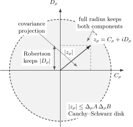
The centered overlap is $z_\rho=C_\rho+iD_\rho$. Cauchy–Schwarz bounds its radius by $\Delta_\rho A\,\Delta_\rho B$. Keeping both projections gives the Robertson–Schrödinger relation; keeping only the vertical commutator projection gives Robertson.

The picture also explains why a vanishing commutator expectation need not make the stronger bound trivial. The point may lie on the real axis with $C_\rho(A,B)\ne0$.

Equality Conditions

Equality deserves separate treatment because there are two inequalities, and their saturation conditions differ.

Pure states and the stronger relation

For a pure state with nonzero variances, Cauchy–Schwarz is saturated exactly when the fluctuation vectors are linearly dependent. There must be a complex number $\lambda$ such that

$$\delta_\psi A|\psi\rangle = \lambda\, \delta_\psi B|\psi\rangle.$$

Equivalently,

$$\left( \delta_\psi A - \lambda\delta_\psi B \right) |\psi\rangle =0.$$

These states are often called intelligent states for the pair $A,B$. The name refers to saturation of a chosen uncertainty relation; it does not imply minimum variance for every observable or minimum energy.

Taking norms shows

$$|\lambda| = \frac{\Delta_\psi A}{\Delta_\psi B}.$$

The real part of $\lambda$ encodes covariance, while its imaginary part encodes the commutator contribution.

Pure states and Robertson alone

Saturating the stronger relation is not enough to saturate the weaker Robertson form. Robertson equality also requires

$$C_\psi(A,B)=0.$$

For nonzero variances, this means the proportionality constant can be chosen purely imaginary:

$$\delta_\psi A|\psi\rangle = i\kappa\, \delta_\psi B|\psi\rangle, \qquad \kappa\in\mathbb R.$$

Thus a correlated Gaussian can saturate Robertson–Schrödinger without saturating Robertson.

Mixed states

In the Hilbert–Schmidt proof, equality holds when

$$\delta_\rho A\sqrt\rho = \lambda\, \delta_\rho B\sqrt\rho$$

for some complex $\lambda$, modulo zero-norm operators. Equivalently,

$$\left( \delta_\rho A - \lambda\delta_\rho B \right) \sqrt\rho =0.$$

This requires linear dependence on the support of $\rho$. For a full-rank state, it is highly restrictive because the relation must hold across the entire Hilbert space.

Zero-variance cases

If $\Delta_\rho A=0$, then

$$\delta_\rho A\sqrt\rho=0.$$

Cauchy–Schwarz then forces

$$C_\rho(A,B)=0, \qquad \langle[A,B]\rangle_\rho=0.$$

The uncertainty relation is saturated trivially. For a pure state, this is the familiar statement that $|\psi\rangle$ is an eigenstate of $A$. It does not make $A$ and $B$ commuting observables.

Worked Example: Two Pauli Components

Let

$$A=\sigma_x, \qquad B=\sigma_z,$$

and write a qubit state as

$$\rho = \frac12 \left( I+\mathbf r\cdot\boldsymbol\sigma \right), \qquad |\mathbf r|\le1.$$

The variances are

$$(\Delta_\rho\sigma_x)^2 = 1-r_x^2,$$

and

$$(\Delta_\rho\sigma_z)^2 = 1-r_z^2.$$

Because $\{\sigma_x,\sigma_z\}=0$,

$$C_\rho(\sigma_x,\sigma_z) = -r_xr_z.$$

Because

$$[\sigma_x,\sigma_z] = -2i\sigma_y,$$

the antisymmetric component is

$$D_\rho(\sigma_x,\sigma_z) = -r_y.$$

The stronger uncertainty relation becomes

$$\begin{aligned} (1-r_x^2)(1-r_z^2) &\ge r_x^2r_z^2+r_y^2. \end{aligned}$$

Subtracting the right side from the left gives

$$1-r_x^2-r_y^2-r_z^2 = 1-|\mathbf r|^2 \ge0.$$

Thus the inequality is exactly the positivity condition for a qubit density operator in this example. Every pure qubit state, for which $|\mathbf r|=1$, saturates the Robertson–Schrödinger relation for this pair. Robertson alone need not be saturated because the covariance $-r_xr_z$ can be nonzero.

Worked Example: Angular Momentum

Angular momentum satisfies

$$[J_x,J_y]=i\hbar J_z.$$

Robertson gives

$$\Delta J_x\,\Delta J_y \ge \frac\hbar2 \left\lvert \langle J_z\rangle \right\rvert.$$

In a simultaneous eigenstate $|j,m\rangle$ of $J^2$ and $J_z$,

$$\langle J_z\rangle=m\hbar,$$

and rotational symmetry about the $z$ axis gives

$$(\Delta J_x)^2 = (\Delta J_y)^2 = \frac{\hbar^2}{2} \left[ j(j+1)-m^2 \right].$$

The covariance $C(J_x,J_y)$ vanishes, so the inequality reduces to

$$j(j+1)-m^2 \ge |m|.$$

Indeed,

$$\begin{aligned} &j(j+1)-m^2-|m| \\ &=(j-|m|)(j+|m|+1) \\ &\ge0. \end{aligned}$$

The extremal states $m=\pm j$ saturate the relation. Nonextremal magnetic sublevels generally do not.

Worked Example: Correlated Gaussian Fluctuations

Let dimensionless canonical quadratures satisfy

$$[X,P]=iI.$$

A rotated squeezed pure Gaussian can have covariance matrix

$$\Gamma = \frac12 R(\theta) \begin{pmatrix} e^{-2r}&0\\ 0&e^{2r} \end{pmatrix} R(\theta)^{\mathsf T},$$

where $R(\theta)$ is a real rotation. Its determinant is

$$\det\Gamma = (\Delta X)^2(\Delta P)^2 - C(X,P)^2 = \frac14.$$

The state saturates Robertson–Schrödinger. When the rotated ellipse has $C(X,P)\ne0$, however,

$$\Delta X\,\Delta P > \frac12,$$

so the simpler Robertson product is not saturated. The covariance term tracks the tilt of the uncertainty ellipse. Concrete wave-packet realizations are treated in Minimum-Uncertainty Wave Packets.

Covariance-Matrix Form

For two observables, define the real covariance matrix

$$\Gamma = \begin{pmatrix} (\Delta_\rho A)^2 & C_\rho(A,B)\\ C_\rho(A,B) & (\Delta_\rho B)^2 \end{pmatrix}.$$

The Robertson–Schrödinger relation is

$$\det\Gamma \ge D_\rho(A,B)^2.$$

The determinant is invariant under rotations of the two-dimensional fluctuation coordinates and measures the squared area scale of their covariance ellipse. The commutator supplies the quantum lower bound on that area.

For a list of observables $X_1,\ldots,X_n$, define

$$\Gamma_{jk} = \frac12 \left\langle \left\lbrace \delta_\rho X_j, \delta_\rho X_k \right\rbrace \right\rangle_\rho,$$

and

$$\Omega_{jk} = \frac1{2i} \langle[X_j,X_k]\rangle_\rho.$$

The full Gram-matrix statement is

$$\Gamma+i\Omega\ge0.$$

Every two-observable Robertson–Schrödinger inequality is a $2\times2$ principal-minor consequence of this positive-semidefinite matrix. For three or more observables, the matrix condition can contain information not visible in an isolated pairwise bound.

For canonical quadratures $R_j$ satisfying

$$[R_j,R_k] = i\hbar J_{jk}I,$$

the condition becomes

$$\Gamma + \frac{i\hbar}{2}J \ge0.$$

This matrix form is central in continuous-variable quantum mechanics and Gaussian-state theory.

What the Lower Bound Does and Does Not Say

The bound is state dependent

Even when $[A,B]\ne0$ as an operator, a particular state may satisfy

$$\langle[A,B]\rangle_\rho=0.$$

Robertson then gives only $\Delta A\,\Delta B\ge0$. Covariance may still make the stronger relation informative, but it can vanish as well. This does not establish compatibility.

The inequality need not give the exact minimum

For a constrained family of states, the smallest attainable product can be larger than the Robertson lower bound. Finding an optimal state is a separate variational problem, and the equality equation may have no admissible solution under the imposed boundary conditions or spectral constraints.

Commuting observables still obey a covariance inequality

If $[A,B]=0$, Robertson reduces to a trivial nonnegative bound, while the stronger relation gives

$$(\Delta A)^2(\Delta B)^2 \ge C(A,B)^2.$$

This is the familiar classical covariance Cauchy–Schwarz inequality. For $B=A$, it is saturated identically.

One observable can be perfectly sharp

An eigenstate of $A$ has $\Delta A=0$. The commutator expectation and covariance must then vanish in that state, even if $A$ and $B$ do not commute as operators. The uncertainty relation forbids certain simultaneous spreads; it does not forbid every sharp preparation of either observable separately.

Nonzero standard deviations are not detector noise

$\Delta_\rho A$ is computed from the ideal Born distribution of $A$ in $\rho$. Calibration errors, finite resolution, and sampling uncertainty are additional experimental effects.

Preparation, Measurement, and Disturbance

To test a preparation uncertainty relation, one prepares many systems in the same state. One subensemble can be measured for $A$ and another for $B$. The inequality compares the resulting ideal distributions; it does not require a simultaneous measurement of both observables on one specimen.

An error–disturbance experiment asks a different question:

1. how accurately does an apparatus approximate a target observable;
2. how much does that apparatus change a later observable;
3. which operational metrics define error and disturbance?

Those questions require a measurement model or quantum instrument. The Robertson inequality contains neither. Confusing these settings turns a precise statistical theorem into an ambiguous slogan.

The distinction is developed from the measurement side in Noncommuting Observables and Compatible, Incompatible, and Sequential Measurements.

Canonical Applications

Position and momentum

When

$$[x,p]=i\hbar I,$$

the commutator expectation is state independent and Robertson gives

$$\Delta x\,\Delta p \ge \frac\hbar2.$$

Fourier interpretation, Gaussian equality states, and boundary/domain caveats belong to Position–Momentum Uncertainty.

Energy and time

In ordinary nonrelativistic quantum mechanics, time is usually an external parameter rather than a self-adjoint observable canonically conjugate to the Hamiltonian. One must therefore not substitute “$A=H$, $B=t$” into Robertson without first defining a time observable and its domain.

Energy–time relations instead arise in several inequivalent forms, including dynamical timescale bounds and lifetime–linewidth relations. Their assumptions and interpretations belong to Energy–Time Uncertainty.

Domain-Safe Form for Unbounded Operators

For unbounded $A$ and $B$, the vector form of the proof is often safer than formal operator products. If

$$|\psi\rangle \in \mathcal D(A) \cap \mathcal D(B),$$

and both variances are finite, then the overlap

$$z_\psi = \left\langle \delta_\psi A\,\psi \middle| \delta_\psi B\,\psi \right\rangle$$

is well defined. Cauchy–Schwarz gives

$$(\Delta_\psi A)^2(\Delta_\psi B)^2 \ge |z_\psi|^2.$$

Its real and imaginary parts define weak covariance and weak commutator forms. Writing the imaginary part as

$$\frac1{2i} \langle\psi|[A,B]|\psi\rangle$$

requires enough additional domain control for $AB$ and $BA$ or an explicit quadratic-form interpretation. A dense domain on which a formal commutator is known is not automatically a license to move unbounded operators freely through bras, kets, or traces.

For mixed states with unbounded observables, one likewise must ensure that the weighted products are trace class and that cyclic trace manipulations are valid. The finite-dimensional Hilbert–Schmidt proof should not be copied formally into a divergent setting.

Practical Workflow

For a concrete pair $A,B$ in a state $\rho$:

1. Verify normalization, self-adjointness, and the required domains.
2. Compute $\langle A\rangle_\rho$ and $\langle B\rangle_\rho$.
3. Compute the variances from the centered operators.
4. Evaluate the commutator expectation.
5. Evaluate the symmetrized covariance when Robertson is loose or equality matters.
6. Compare squared quantities in Robertson–Schrödinger to avoid premature square roots.
7. Check dimensions and simple limiting cases.
8. If equality is claimed, verify linear dependence of the centered fluctuation vectors.
9. Keep measurement error and disturbance outside the calculation unless an instrument has been specified.

Common Mistakes

• Calling every uncertainty relation “Heisenberg’s inequality” without stating which mathematical form is meant.
• Omitting the covariance term while claiming the strongest two-observable bound.
• Treating $\Delta A$ as a centered operator instead of a nonnegative number.
• Forgetting to center $A$ and $B$ before applying Cauchy–Schwarz.
• Assuming $[A,B]\ne0$ guarantees a positive Robertson lower bound in every state.
• Assuming a zero Robertson lower bound means both variances can vanish.
• Treating equality in Robertson–Schrödinger as equality in Robertson.
• Calling every saturating state a minimum-energy or coherent state.
• Interpreting preparation spread as apparatus error or sequential disturbance.
• Applying an energy–time slogan as though time were automatically an observable conjugate to $H$.
• Ignoring covariance, units, divergent moments, or unbounded-operator domains.
• Taking square roots before confirming that all quantities are real and nonnegative.

Canonical Boundaries

This page owns the Cauchy–Schwarz derivation, the covariance-strengthened relation, equality conditions, and the multi-observable Gram-matrix form. Nearby pages own the supporting and specialized material:

• Variance and Standard Deviation owns moments, statistical spread, and finite-variance conditions.
• Correlations and Covariance owns symmetrized covariance and quantum correlation conventions.
• Anticommutators owns the symmetric operator product and its broader uses.
• Commutators owns bracket algebra and generator identities.
• Position–Momentum Uncertainty owns the canonical wave-mechanics specialization.
• Energy–Time Uncertainty owns dynamical timescale and lifetime–linewidth relations.

Summary

• Variances are squared norms of centered fluctuation vectors.
• Cauchy–Schwarz bounds their product by the squared magnitude of their centered overlap.
• The real part of that overlap is symmetrized covariance.
• The imaginary part is one half of the commutator expectation divided by $i$.
• Keeping both parts gives Robertson–Schrödinger; dropping covariance gives Robertson.
• The stronger relation is a determinant bound on the covariance matrix.
• Pure-state equality requires linearly dependent centered fluctuation vectors.
• Robertson equality additionally requires zero symmetrized covariance.
• A vanishing state-dependent lower bound does not imply commuting observables.
• Preparation uncertainty is distinct from measurement error and disturbance.
• Unbounded observables require domain-aware vector or quadratic-form statements.

References

• E. H. Kennard, “Zur Quantenmechanik einfacher Bewegungstypen,” Zeitschrift für Physik 44, 326–352, 1927, doi:10.1007/BF01391200.
• H. P. Robertson, “The Uncertainty Principle,” Physical Review 34, 163–164, 1929, doi:10.1103/PhysRev.34.163.
• E. Schrödinger, “Zum Heisenbergschen Unschärfeprinzip,” Sitzungsberichte der Preußischen Akademie der Wissenschaften, Physikalisch-mathematische Klasse, 296–303, 1930.
• P. A. M. Dirac, The Principles of Quantum Mechanics, 4th ed., Oxford University Press, 1958.
• A. Peres, Quantum Theory: Concepts and Methods, Kluwer, 1995.
• R. Shankar, Principles of Quantum Mechanics, 2nd ed., Springer, 1994.
• J. J. Sakurai and J. Napolitano, Modern Quantum Mechanics, 3rd ed., Cambridge University Press, 2020.
• B. C. Hall, Quantum Theory for Mathematicians, Springer, 2013.
• R. Simon, N. Mukunda, and B. Dutta, “Quantum-Noise Matrix for Multimode Systems: U(n) Invariance, Squeezing, and Normal Forms,” Physical Review A 49, 1567–1583, 1994, doi:10.1103/PhysRevA.49.1567.
• V. V. Dodonov, “Purity- and Entropy-Bounded Uncertainty Relations for Mixed Quantum States,” Journal of Optics B: Quantum and Semiclassical Optics 4, S98–S108, 2002.
• P. Busch, P. Lahti, J.-P. Pellonpää, and K. Ylinen, Quantum Measurement, Springer, 2016.

Exercises

Exercise 1: Centered covariance identity

Starting from

$$C_\rho(A,B) = \frac12 \left\langle \left\lbrace \delta_\rho A, \delta_\rho B \right\rbrace \right\rangle_\rho,$$

show that

$$C_\rho(A,B) = \frac12\langle\{A,B\}\rangle_\rho - \langle A\rangle_\rho \langle B\rangle_\rho.$$

Solution

Write $a=\langle A\rangle_\rho$ and $b=\langle B\rangle_\rho$. Then

$$\begin{aligned} \{A-aI,B-bI\} &= \{A,B\} -2bA \\ &\quad-2aB +2abI. \end{aligned}$$

Taking the expectation gives

$$\begin{aligned} \left\langle \{\delta_\rho A,\delta_\rho B\} \right\rangle_\rho &= \langle\{A,B\}\rangle_\rho -2ab. \end{aligned}$$

Dividing by two yields

$$C_\rho(A,B) = \frac12\langle\{A,B\}\rangle_\rho-ab.$$

Exercise 2: Mixed-state derivation

Let

$$X=\delta_\rho A\sqrt\rho, \qquad Y=\delta_\rho B\sqrt\rho.$$

Use Hilbert–Schmidt Cauchy–Schwarz to derive the Robertson–Schrödinger relation without assuming that $\rho$ is pure.

Solution

Hilbert–Schmidt Cauchy–Schwarz gives

$$(X,X)_{\mathrm{HS}}(Y,Y)_{\mathrm{HS}} \ge |(X,Y)_{\mathrm{HS}}|^2.$$

The diagonal terms are

$$\begin{aligned} (X,X)_{\mathrm{HS}} &=(\Delta_\rho A)^2,\\ (Y,Y)_{\mathrm{HS}} &=(\Delta_\rho B)^2. \end{aligned}$$

The overlap is

$$(X,Y)_{\mathrm{HS}} = \left\langle \delta_\rho A\,\delta_\rho B \right\rangle_\rho = C_\rho+iD_\rho.$$

Therefore

$$\begin{aligned} (\Delta_\rho A)^2(\Delta_\rho B)^2 &\ge C_\rho(A,B)^2 \\ &\quad+ \frac14 \left\lvert \langle[A,B]\rangle_\rho \right\rvert^2. \end{aligned}$$

Exercise 3: Stronger equality without Robertson equality

For $A=\sigma_x$, $B=\sigma_z$, take the pure qubit state with Bloch vector

$$\mathbf r = \frac1{\sqrt2}(1,0,1).$$

Compute the two variances, covariance, and commutator expectation. Show that Robertson–Schrödinger is saturated while Robertson is not.

Solution

Here

$$r_x=r_z=\frac1{\sqrt2}, \qquad r_y=0.$$

Thus

$$(\Delta\sigma_x)^2 = (\Delta\sigma_z)^2 = \frac12.$$

The covariance is

$$C(\sigma_x,\sigma_z) = -r_xr_z = -\frac12,$$

while

$$\langle[\sigma_x,\sigma_z]\rangle = -2i\langle\sigma_y\rangle =0.$$

The squared left side is

$$(\Delta\sigma_x)^2(\Delta\sigma_z)^2 = \frac14,$$

and the stronger right side is

$$C^2+\frac14|\langle[\sigma_x,\sigma_z]\rangle|^2 = \frac14.$$

So Robertson–Schrödinger is saturated. Robertson reads

$$\Delta\sigma_x\,\Delta\sigma_z = \frac12 > 0,$$

and is not saturated.

Exercise 4: Extremal angular-momentum states

For $|j,m\rangle$, use

$$(\Delta J_x)^2 = (\Delta J_y)^2 = \frac{\hbar^2}{2} \left[j(j+1)-m^2\right]$$

to show that the $J_x,J_y$ Robertson inequality is saturated exactly for $m=\pm j$, apart from the trivial $j=0$ case.

Solution

Because the variances are equal,

$$\Delta J_x\,\Delta J_y = \frac{\hbar^2}{2} \left[j(j+1)-m^2\right].$$

The Robertson lower bound is

$$\frac12 \left\lvert \langle[J_x,J_y]\rangle \right\rvert = \frac{\hbar^2}{2}|m|.$$

Their difference, after removing the common factor $\hbar^2/2$, is

$$\begin{aligned} &j(j+1)-m^2-|m| \\ &=(j-|m|)(j+|m|+1). \end{aligned}$$

For allowed magnetic quantum numbers, both factors are nonnegative. The first vanishes exactly when $|m|=j$. Thus the extremal states saturate.

Exercise 5: Zero variance constrains both overlap terms

Suppose $\Delta_\rho A=0$. Prove directly from $\delta_\rho A\sqrt\rho=0$ that

$$C_\rho(A,B)=0, \qquad \langle[A,B]\rangle_\rho=0$$

for every bounded observable $B$.

Solution

The variance is the Hilbert–Schmidt norm

$$(\Delta_\rho A)^2 = \left\lVert \delta_\rho A\sqrt\rho \right\rVert_{\mathrm{HS}}^2.$$

If it vanishes, then

$$\delta_\rho A\sqrt\rho=0.$$

Hence its Hilbert–Schmidt inner product with $\delta_\rho B\sqrt\rho$ is zero:

$$\left\langle \delta_\rho A\,\delta_\rho B \right\rangle_\rho =0.$$

The real and imaginary parts of this complex number are respectively $C_\rho(A,B)$ and $\langle[A,B]\rangle_\rho/(2i)$. Both must vanish.

Exercise 6: Commuting observables and classical covariance

Assume $[A,B]=0$. Show that Robertson–Schrödinger reduces to

$$|C_\rho(A,B)| \le \Delta_\rho A\,\Delta_\rho B.$$

When $\Delta_\rho A$ and $\Delta_\rho B$ are nonzero, define

$$r_{AB} = \frac{C_\rho(A,B)} {\Delta_\rho A\,\Delta_\rho B}.$$

What range can $r_{AB}$ take, and when is equality possible?

Solution

With a zero commutator, the stronger relation becomes

$$(\Delta_\rho A)^2(\Delta_\rho B)^2 \ge C_\rho(A,B)^2.$$

Taking nonnegative square roots gives the stated covariance bound. Dividing by the positive standard deviations yields

$$-1\le r_{AB}\le1.$$

Equality occurs when the centered fluctuations are linearly dependent on the support of the state. In a common eigenbasis, this is the ordinary condition that the two centered random variables are perfectly linearly correlated or anticorrelated on outcomes of nonzero probability.

Exercise 7: Positivity of the uncertainty matrix

For observables $X_1,\ldots,X_n$, define

$$G_{jk} = \left\langle \delta_\rho X_j\, \delta_\rho X_k \right\rangle_\rho.$$

Show that $G=\Gamma+i\Omega$ is positive semidefinite.

Solution

For arbitrary complex coefficients $c_1,\ldots,c_n$, let

$$Y = \sum_kc_k\delta_\rho X_k.$$

Then

$$\begin{aligned} \sum_{j,k}c_j^{*}G_{jk}c_k &= \left\langle Y^{\dagger}Y \right\rangle_\rho \\ &\ge0. \end{aligned}$$

Therefore $G\ge0$. Splitting each entry into the expectation of an anticommutator and a commutator gives

$$G_{jk} = \Gamma_{jk} + i\Omega_{jk}.$$

Hence $\Gamma+i\Omega\ge0$.

Exercise 8: A domain-safe weak commutator

Let $A$ and $B$ be self-adjoint and let $|\psi\rangle\in\mathcal D(A)\cap\mathcal D(B)$. Define

$$w_\psi(A,B) = \langle A\psi|B\psi\rangle - \langle B\psi|A\psi\rangle.$$

Show that $w_\psi(A,B)$ is purely imaginary and that

$$\Delta_\psi A\,\Delta_\psi B \ge \frac12|w_\psi(A,B)|.$$

Why is this formulation safer than writing $\langle\psi|[A,B]|\psi\rangle$ immediately?

Solution

The second term is the complex conjugate of the first, so

$$w_\psi(A,B)^{*} = -w_\psi(A,B).$$

Thus $w_\psi(A,B)$ is purely imaginary. Centering does not change the difference, and Cauchy–Schwarz gives

$$\begin{aligned} \Delta_\psi A\,\Delta_\psi B &\ge \left\lvert \operatorname{Im} \langle\delta_\psi A\,\psi |\delta_\psi B\,\psi\rangle \right\rvert \\ &= \frac12|w_\psi(A,B)|. \end{aligned}$$

The vectors $A|\psi\rangle$ and $B|\psi\rangle$ exist under the stated common domain assumption. By contrast, $AB|\psi\rangle$ and $BA|\psi\rangle$ require the stronger conditions $B|\psi\rangle\in\mathcal D(A)$ and $A|\psi\rangle\in\mathcal D(B)$. The weak form avoids assuming those product domains silently.