Correlations and Covariance

Correlations describe how fluctuations of two observables are related in a specified quantum state. If large outcomes of $A$ tend to occur with large outcomes of $B$, their covariance is positive; if large outcomes of one tend to accompany small outcomes of the other, it is negative. Zero covariance means only that there is no linear correlation of this kind.

For a state $\rho$, define centered observables

$$\delta_\rho A \equiv A-\langle A\rangle_\rho I, \qquad \delta_\rho B \equiv B-\langle B\rangle_\rho I.$$

The standard real covariance of two self-adjoint observables is

$$\operatorname{Cov}_\rho(A,B) \equiv \frac12 \left\langle \delta_\rho A\,\delta_\rho B + \delta_\rho B\,\delta_\rho A \right\rangle_\rho.$$

The symmetrization is invisible for commuting observables. For noncommuting observables it is essential: an ordered product such as $\langle AB\rangle$ can be complex and is not automatically an ordinary joint-outcome moment.

This page owns static two-observable covariance in finite systems and the first encounter with connected correlations. Generic probability covariance belongs at Variance and Covariance, while time ordering and response functions belong to Quantum Dynamics and Formulations and correlation lengths and cluster decomposition to Many-Body and Quantum Statistical Mechanics. No result on this page depends on those extensions.

Required background. Expectation Values supplies operator moments; Variance and Standard Deviation supplies centered observables and spread.

Helpful background. Commutators explains why ordering matters for noncommuting observables.

Paired fluctuations

For classical random variables with a joint distribution, covariance is

$$\operatorname{Cov}(A,B) = \mathbb E\!\left[ (A-\mathbb E[A])(B-\mathbb E[B]) \right].$$

The sign is determined by paired deviations from the means. Outcomes in the same-sign quadrants contribute positively; outcomes in opposite-sign quadrants contribute negatively.

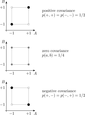
For centered binary outcomes $A,B=\pm1$, weight on the equal-sign pairs gives positive covariance, uniform weight gives zero covariance, and weight on the opposite-sign pairs gives negative covariance. These are ordinary joint distributions and therefore model compatible or separately localized measurements.

Covariance depends on the pairing. Knowing the separate marginal distributions of $A$ and $B$ is not enough to determine it.

Compatible observables and joint probabilities

For finite-dimensional commuting observables,

$$[A,B]=0,$$

their spectral projectors commute and define a joint projective measurement. If $P_a^A$ and $P_b^B$ are the spectral projectors, then

$$p_\rho(a,b) = \operatorname{Tr}\!\left( \rho P_a^A P_b^B \right).$$

The projectors $P_a^AP_b^B$ are mutually orthogonal, positive, and sum to the identity over all joint outcomes. The marginals are

$$\begin{aligned} p_\rho^A(a)&=\sum_b p_\rho(a,b),\\ p_\rho^B(b)&=\sum_a p_\rho(a,b). \end{aligned}$$

The covariance is then the ordinary joint-distribution statistic

$$\begin{aligned} \operatorname{Cov}_\rho(A,B) &= \sum_{a,b}(a-\langle A\rangle_\rho)\\ &\quad{} \times(b-\langle B\rangle_\rho) p_\rho(a,b). \end{aligned}$$

In infinite-dimensional settings, the precise compatibility condition is commutation of the spectral measures, often called strong commutativity. Formal commutators of unbounded operators require domain care and do not by themselves replace that spectral condition.

Symmetrized covariance

Expanding the centered observables gives

$$\begin{aligned} \operatorname{Cov}_\rho(A,B) &= \frac12\langle AB+BA\rangle_\rho\\ &\quad- \langle A\rangle_\rho \langle B\rangle_\rho. \end{aligned}$$

Equivalently, using the anticommutator $\{A,B\}=AB+BA$,

$$\operatorname{Cov}_\rho(A,B) = \frac12\langle\{A,B\}\rangle_\rho - \langle A\rangle_\rho \langle B\rangle_\rho.$$

The covariance is real and symmetric:

$$\operatorname{Cov}_\rho(A,B) = \operatorname{Cov}_\rho(B,A) \in\mathbb R.$$

It reduces to variance on the diagonal:

$$\operatorname{Cov}_\rho(A,A) = \operatorname{Var}_\rho(A).$$

The commutator and anticommutator split is developed algebraically at Commutators and Anticommutators. The Hermitian symmetric-product interpretation is developed in Anticommutators.

Ordered covariance and the commutator

The ordered centered product is

$$C_\rho(A,B) \equiv \left\langle \delta_\rho A\,\delta_\rho B \right\rangle_\rho.$$

It decomposes as

$$C_\rho(A,B) = \operatorname{Cov}_\rho(A,B) + \frac12\langle[A,B]\rangle_\rho.$$

For self-adjoint $A$ and $B$, the covariance is real and $\langle[A,B]\rangle_\rho$ is purely imaginary whenever the expressions are defined. Thus

$$\begin{aligned} \operatorname{Re}C_\rho(A,B) &= \operatorname{Cov}_\rho(A,B),\\ \operatorname{Im}C_\rho(A,B) &= \frac{1}{2i}\langle[A,B]\rangle_\rho. \end{aligned}$$

The real part describes symmetrized fluctuation alignment. The imaginary part records noncommutativity. Neither statement creates a simultaneous sharp joint distribution for incompatible observables.

Quadratic-form definition

For a pure state and possibly unbounded observables, a safer definition uses the centered vectors

$$|f_A\rangle = \delta_\psi A|\psi\rangle, \qquad |f_B\rangle = \delta_\psi B|\psi\rangle.$$

If $|\psi\rangle\in D(A)\cap D(B)$ and both variances are finite, define

$$\operatorname{Cov}_\psi(A,B) = \operatorname{Re}\langle f_A|f_B\rangle.$$

This requires the vectors $A|\psi\rangle$ and $B|\psi\rangle$, but it does not automatically require $AB|\psi\rangle$ or $BA|\psi\rangle$ to exist. The anticommutator expression should be interpreted through this quadratic form when operator-product domains are problematic.

Correlation coefficient

When both standard deviations are nonzero, define

$$r_\rho(A,B) = \frac{ \operatorname{Cov}_\rho(A,B) }{ \Delta_\rho A\,\Delta_\rho B }.$$

Cauchy–Schwarz gives

$$|r_\rho(A,B)|\le1.$$

The coefficient is dimensionless and invariant under positive affine rescalings. Its sign reverses if exactly one observable is multiplied by a negative number.

The interpretations are limited but useful:

• $r=1$ means the centered operator-state vectors saturate Cauchy–Schwarz with positive proportionality.
• $r=-1$ means they saturate it with negative proportionality.
• $r=0$ means zero symmetrized linear covariance.

Only when $A$ and $B$ admit a joint probability law do the first two cases reduce to the classical statement of a perfectly aligned or anti-aligned linear relation between random variables.

If either variance vanishes, $r$ is undefined rather than zero. In that case the corresponding observable has no fluctuations to normalize.

Zero covariance is not independence

Statistical independence implies factorization of every suitable product moment for a joint distribution, and hence zero covariance. The converse is false. A nonlinear dependence can have zero covariance.

In quantum mechanics, zero symmetrized covariance is even less restrictive:

• It does not imply that $A$ and $B$ commute.
• It does not imply a joint sharp probability distribution.
• It does not imply that two subsystems are in a product state.
• It does not rule out higher-order or nonlinear correlations.

A single number cannot certify absence of correlation structure.

Covariance matrices

For self-adjoint observables $A_1,\ldots,A_n$, define the real covariance matrix

$$\Gamma_{jk} \equiv \frac12 \left\langle \delta A_j\delta A_k + \delta A_k\delta A_j \right\rangle.$$

It is real and symmetric. Its diagonal entries are variances:

$$\Gamma_{jj} = (\Delta A_j)^2.$$

For any real vector $\mathbf c$,

$$\begin{aligned} \mathbf c^{\mathsf T}\Gamma\mathbf c &= \operatorname{Var}\!\left( \sum_j c_jA_j \right)\\ &\ge0. \end{aligned}$$

Hence $\Gamma$ is positive semidefinite. Every $2\times2$ principal minor is nonnegative, yielding

$$\operatorname{Cov}(A,B)^2 \le \operatorname{Var}(A)\operatorname{Var}(B),$$

which is the bound behind $|r|\le1$.

Linear changes of observables

For real coefficients,

$$\begin{aligned} &\operatorname{Cov}(\alpha A+\beta I,\gamma B+\eta I)\\ &\qquad= \alpha\gamma\operatorname{Cov}(A,B). \end{aligned}$$

Constant shifts disappear after centering. For a vector of observables $\mathbf A$ transformed by a real matrix $M$,

$$\mathbf A'=M\mathbf A,$$

the covariance matrix transforms as

$$\Gamma'=M\Gamma M^{\mathsf T}.$$

This rule is useful for changing quadratures, rotating spin components, or forming collective observables.

Recovering covariance from variances

Expanding the variance of a sum gives the polarization identity

$$\begin{aligned} \operatorname{Var}(A+B) &= \operatorname{Var}(A)+\operatorname{Var}(B)\\ &\quad+ 2\operatorname{Cov}(A,B). \end{aligned}$$

Therefore

$$\begin{aligned} 2\operatorname{Cov}(A,B) &= \operatorname{Var}(A+B)-\operatorname{Var}(A)\\ &\quad- \operatorname{Var}(B). \end{aligned}$$

An equivalent symmetric form is

$$\begin{aligned} 4\operatorname{Cov}(A,B) &= \operatorname{Var}(A+B)\\ &\quad- \operatorname{Var}(A-B). \end{aligned}$$

These identities remain valid for noncommuting observables because variance of $A\pm B$ automatically contains the symmetrized cross term. They also suggest an operational route: estimate variances of the separately implemented observables $A+B$ and $A-B$, rather than claiming a simultaneous sharp measurement of $A$ and $B$.

Connected correlations

The ordered connected two-point function is

$$\langle AB\rangle_{\rho,c} \equiv \langle AB\rangle_\rho - \langle A\rangle_\rho \langle B\rangle_\rho.$$

For commuting observables this equals their covariance. For noncommuting observables it is order dependent and may be complex:

$$\langle AB\rangle_{\rho,c} = \operatorname{Cov}_\rho(A,B) + \frac12\langle[A,B]\rangle_\rho.$$

One must state whether a problem uses $\langle AB\rangle_c$, $\langle BA\rangle_c$, a symmetrized correlator, a time-ordered correlator, or a retarded commutator. These objects answer different physical questions.

Connected Correlation Functions owns cumulants, cluster decomposition, spatial decay, and the many-body meaning of connectedness.

Local observables on two subsystems

For a bipartite system, local observables

$$A_1=A\otimes I, \qquad B_2=I\otimes B$$

commute. Their product is

$$A_1B_2=A\otimes B,$$

so the local covariance is

$$\begin{aligned} \operatorname{Cov}_\rho(A_1,B_2) &= \langle A\otimes B\rangle_\rho\\ &\quad- \langle A\otimes I\rangle_\rho \langle I\otimes B\rangle_\rho. \end{aligned}$$

For a product state $\rho=\rho_1\otimes\rho_2$, all such local product expectations factorize, so every local covariance vanishes. A separable mixture can nevertheless have nonzero local covariance because the classical mixing variable correlates the subsystems.

The full relation among marginals, classical correlations, and entanglement is developed at Marginals and Correlations.

Example: Bell-state correlations

Consider

$$|\Phi^+\rangle = \frac{|00\rangle+|11\rangle}{\sqrt2}.$$

For

$$A=Z\otimes I, \qquad B=I\otimes Z,$$

the local means vanish,

$$\langle A\rangle=\langle B\rangle=0,$$

while

$$\langle AB\rangle = \langle Z\otimes Z\rangle =1.$$

Thus

$$\operatorname{Cov}(A,B)=1, \qquad r(A,B)=1.$$

The local outcomes are individually random and perfectly correlated.

Correlation alone does not certify entanglement

The separable mixed state

$$\rho_{\mathrm{cc}} = \frac12|00\rangle\langle00| + \frac12|11\rangle\langle11|$$

has the same $Z$ statistics:

$$\begin{aligned} \langle Z\otimes I\rangle&=0,\\ \langle I\otimes Z\rangle&=0,\\ \langle Z\otimes Z\rangle&=1. \end{aligned}$$

Therefore its $Z$ covariance is also one. The Bell state and this separable state differ in other measurement bases and in their coherence, but one covariance cannot distinguish them. See Classical Correlation versus Entanglement for the canonical distinction.

Example: noncommuting Pauli observables

Take $|+z\rangle$ and let

$$A=\sigma_x, \qquad B=\sigma_y.$$

The means vanish, and the anticommutator is zero:

$$\langle\sigma_x\rangle = \langle\sigma_y\rangle=0, \qquad \{\sigma_x,\sigma_y\}=0.$$

Hence

$$\operatorname{Cov}(\sigma_x,\sigma_y)=0.$$

But

$$\begin{aligned} \langle\sigma_x\sigma_y\rangle &= i\langle\sigma_z\rangle=i,\\ \langle\sigma_y\sigma_x\rangle &=-i. \end{aligned}$$

The zero real covariance does not imply compatibility. The imaginary ordered part records

$$[\sigma_x,\sigma_y] = 2i\sigma_z.$$

Example: position–momentum covariance

For one-dimensional position and momentum,

$$\operatorname{Cov}(X,P) = \frac12\langle XP+PX\rangle - \langle X\rangle\langle P\rangle.$$

It measures the linear tilt of phase-space fluctuations. Consider the chirped Gaussian

$$\begin{aligned} \xi &=x-x_0,\\ \psi(x) &= \frac{1}{(2\pi s^2)^{1/4}} \exp\!\left[ -\frac{1-i\kappa}{4s^2}\xi^2 \right]\\ &\quad{} \times \exp\!\left[ \frac{ip_0\xi}{\hbar} \right]. \end{aligned}$$

Its moments are

$$\begin{aligned} (\Delta X)^2&=s^2,\\ \operatorname{Cov}(X,P)&=\frac{\hbar\kappa}{2},\\ (\Delta P)^2&= \frac{\hbar^2}{4s^2}(1+\kappa^2). \end{aligned}$$

The covariance vanishes for an unchirped packet and changes sign with $\kappa$. The determinant obeys

$$(\Delta X)^2(\Delta P)^2 - \operatorname{Cov}(X,P)^2 = \frac{\hbar^2}{4},$$

so this pure Gaussian saturates the Schrödinger uncertainty relation.

Covariance and uncertainty

For a pure state, Cauchy–Schwarz applied to $|f_A\rangle$ and $|f_B\rangle$ gives the Schrödinger–Robertson inequality

$$\begin{aligned} (\Delta A)^2(\Delta B)^2 &\ge \operatorname{Cov}(A,B)^2\\ &\quad+ \frac14 \left| \langle[A,B]\rangle \right|^2. \end{aligned}$$

The covariance term is the real part of the centered overlap, and the commutator term is its imaginary part. Dropping the nonnegative covariance term gives the weaker Robertson bound. The canonical derivation and equality conditions are at General Uncertainty Relations.

From static covariance to correlation functions

Many-body and dynamical applications attach positions, sites, components, or times to the observables:

$$C_{AB}(i,j;t,t') = \langle A_i(t)B_j(t')\rangle.$$

Ordering then becomes physical. Equal-time commuting local observables, time-ordered products, symmetrized noise correlators, and retarded commutators are not interchangeable. This page supplies the static centered-product language only.

The roadmap to those choices is Correlation Functions Overview.

Common mistakes

Calling every product expectation a covariance

$\langle AB\rangle$ contains the disconnected product of means. Subtract $\langle A\rangle\langle B\rangle$ when a connected correlation is intended.

Ignoring operator order

For noncommuting observables, $\langle AB\rangle$ and $\langle BA\rangle$ can differ. State the ordering or symmetrization convention.

Assuming a joint distribution for incompatible observables

The symmetrized covariance is well defined without an ordinary simultaneous sharp joint measurement. Do not interpret it as a classical joint moment unless a compatible measurement construction has been specified.

Equating zero covariance with independence

Zero covariance removes one linear second-order statistic. It does not remove higher-order, nonlinear, quantum, or entanglement correlations.

Equating correlation with entanglement

Separable mixed states can have strong classical correlations. Entanglement requires criteria involving the full bipartite state or a suitable witness.

Normalizing by a zero standard deviation

The correlation coefficient is undefined if either observable has zero variance. Covariance itself remains meaningful and is then zero.

Neglecting domains

For unbounded observables, $AB$ and $BA$ may not be defined on the state even when $A|\psi\rangle$ and $B|\psi\rangle$ are. Use the quadratic-form definition and state the required domain assumptions.

Summary

For self-adjoint observables, the real symmetrized covariance is

$$\operatorname{Cov}_\rho(A,B) = \frac12 \left\langle \{\delta_\rho A,\delta_\rho B\} \right\rangle_\rho.$$

It is the ordinary covariance of a joint Born distribution when the sharp observables are compatible. For noncommuting observables it equals the real part of the ordered centered product, while the commutator supplies the imaginary part. Covariance matrices are positive semidefinite, the normalized coefficient obeys $|r|\le1$, and zero covariance does not imply independence, compatibility, or absence of entanglement. Connected and ordered correlation functions must always state their subtraction and ordering conventions.

References

• L. E. Ballentine, Quantum Mechanics: A Modern Development, 2nd ed., World Scientific, 2014, Chapters 2–3.
• M. A. Nielsen and I. L. Chuang, Quantum Computation and Quantum Information, 10th anniversary ed., Cambridge University Press, 2010, Chapters 2 and 12.
• H. P. Robertson, “The Uncertainty Principle,” Physical Review 34, 163–164 (1929).
• J. J. Sakurai and J. Napolitano, Modern Quantum Mechanics, 3rd ed., Cambridge University Press, 2020, Chapters 1–2.
• E. Schrödinger, “Zum Heisenbergschen Unschärfeprinzip,” Sitzungsberichte der Preussischen Akademie der Wissenschaften, Physikalisch-mathematische Klasse, 296–303 (1930).
• R. Shankar, Principles of Quantum Mechanics, 2nd ed., Springer, 1994, Chapters 1 and 4.
• J. von Neumann, Mathematical Foundations of Quantum Mechanics, Princeton University Press, 1955, Chapters II–III.

Exercises

1. Covariance with itself

Show directly from the symmetrized definition that

$$\operatorname{Cov}_\rho(A,A) = \operatorname{Var}_\rho(A).$$

Solution

Setting $B=A$ gives

$$\begin{aligned} \operatorname{Cov}_\rho(A,A) &= \frac12 \langle\delta A\delta A+\delta A\delta A\rangle_\rho\\ &= \langle(\delta A)^2\rangle_\rho\\ &= \operatorname{Var}_\rho(A). \end{aligned}$$

2. A binary joint distribution

Two commuting observables have outcomes $A,B=\pm1$ with

$$p(+,+)=p(-,-)=\frac{1+c}{4},$$

and

$$p(+,-)=p(-,+)=\frac{1-c}{4},$$

where $-1\le c\le1$. Find the means, variances, covariance, and correlation coefficient.

Solution

Each marginal is uniform, so

$$\begin{aligned} \langle A\rangle=\langle B\rangle&=0,\\ \operatorname{Var}(A)=\operatorname{Var}(B)&=1. \end{aligned}$$

The product $AB$ is $+1$ for equal signs and $-1$ for opposite signs. Hence

$$\begin{aligned} \langle AB\rangle &= 2\frac{1+c}{4} - 2\frac{1-c}{4}\\ &=c. \end{aligned}$$

Because the means vanish,

$$\operatorname{Cov}(A,B)=c, \qquad r(A,B)=c.$$

3. Bell-state covariance

For $|\Phi^+\rangle=(|00\rangle+|11\rangle)/\sqrt2$, calculate the covariance and correlation coefficient of $A=Z\otimes I$ and $B=I\otimes Z$.

Solution

Each local outcome is $\pm1$ with equal probability, so

$$\langle A\rangle=\langle B\rangle=0, \qquad \Delta A=\Delta B=1.$$

The outcomes always have equal signs, and

$$\langle AB\rangle = \langle Z\otimes Z\rangle =1.$$

Therefore

$$\operatorname{Cov}(A,B)=1, \qquad r(A,B)=1.$$

4. Correlation without entanglement

For

$$\rho_{\mathrm{cc}} = \frac12|00\rangle\langle00| + \frac12|11\rangle\langle11|,$$

compute the same $Z$ covariance as in Exercise 3. Why does the result not certify entanglement?

Solution

The local means vanish and every preparation gives equal $Z$ signs, so

$$\langle Z\otimes Z\rangle=1$$

and the covariance is $1$. But $\rho_{\mathrm{cc}}$ is explicitly a convex mixture of the product states $|00\rangle$ and $|11\rangle$. It is separable. The covariance detects correlation in this measurement basis, not the source of that correlation.

5. Noncommuting Pauli pair

In the state $|+z\rangle$, evaluate

$$C(\sigma_x,\sigma_y) = \langle\delta\sigma_x\delta\sigma_y\rangle,$$

its real covariance, and its commutator contribution.

Solution

Both means vanish, so the centered operators equal the original operators. Using $\sigma_x\sigma_y=i\sigma_z$,

$$C(\sigma_x,\sigma_y) = i\langle\sigma_z\rangle =i.$$

The real part is zero:

$$\operatorname{Cov}(\sigma_x,\sigma_y)=0.$$

The commutator contribution is

$$\frac12\langle[\sigma_x,\sigma_y]\rangle = \frac12\langle2i\sigma_z\rangle =i.$$

6. Polarization from variances

Prove that

$$\begin{aligned} 4\operatorname{Cov}(A,B) &= \operatorname{Var}(A+B)\\ &\quad- \operatorname{Var}(A-B) \end{aligned}$$

without assuming that $A$ and $B$ commute.

Solution

Centering is linear:

$$\delta(A\pm B)=\delta A\pm\delta B.$$

Therefore

$$\begin{aligned} \operatorname{Var}(A+B) &= \operatorname{Var}(A)+\operatorname{Var}(B)\\ &\quad+2\operatorname{Cov}(A,B),\\ \operatorname{Var}(A-B) &= \operatorname{Var}(A)+\operatorname{Var}(B)\\ &\quad-2\operatorname{Cov}(A,B). \end{aligned}$$

Subtracting the second equation from the first gives the result. The cross terms enter as $\delta A\delta B+\delta B\delta A$, so no commutativity assumption is needed.

7. Positivity of a two-observable covariance matrix

Let

$$\Gamma = \begin{pmatrix} (\Delta A)^2 & \operatorname{Cov}(A,B)\\ \operatorname{Cov}(A,B) & (\Delta B)^2 \end{pmatrix}.$$

Use positivity to derive $|r(A,B)|\le1$ when both variances are nonzero.

Solution

For real $u,v$,

$$\begin{pmatrix}u&v\end{pmatrix} \Gamma \begin{pmatrix}u\\v\end{pmatrix} = \operatorname{Var}(uA+vB) \ge0.$$

Thus $\Gamma$ is positive semidefinite, so its determinant is nonnegative:

$$(\Delta A)^2(\Delta B)^2 - \operatorname{Cov}(A,B)^2 \ge0.$$

Dividing by the positive product of variances gives

$$|r(A,B)| = \frac{|\operatorname{Cov}(A,B)|} {\Delta A\,\Delta B} \le1.$$

8. Chirped Gaussian uncertainty determinant

Suppose a state has

$$(\Delta X)^2=s^2, \qquad \operatorname{Cov}(X,P)=\frac{\hbar\kappa}{2},$$

and

$$(\Delta P)^2 = \frac{\hbar^2}{4s^2}(1+\kappa^2).$$

Evaluate the covariance-corrected uncertainty determinant.

Solution

Substitution gives

$$\begin{aligned} (\Delta X)^2(\Delta P)^2 &= \frac{\hbar^2}{4}(1+\kappa^2),\\ \operatorname{Cov}(X,P)^2 &= \frac{\hbar^2\kappa^2}{4}. \end{aligned}$$

Therefore

$$(\Delta X)^2(\Delta P)^2 - \operatorname{Cov}(X,P)^2 = \frac{\hbar^2}{4}.$$

The chirp increases both momentum variance and position–momentum covariance in exactly the combination needed to preserve saturation of the Schrödinger uncertainty relation.