Probability Amplitudes

A probability amplitude is a complex quantity associated with a specified preparation, transformation, and measurement alternative. In the simplest case, a normalized state $\lvert\psi\rangle$ is tested against a normalized target ray represented by $\lvert\phi\rangle$. The transition amplitude is

$$\mathcal A(\phi\leftarrow\psi) = \langle\phi\rvert\psi\rangle,$$

and the corresponding rank-one projective probability is

$$p(\phi\mid\psi) = \lvert\mathcal A(\phi\leftarrow\psi)\rvert^2.$$

The amplitude is not itself a probability. It can be negative or complex, it depends on phase conventions, and it can interfere with other amplitudes. Only after the physical alternatives and the measurement are specified does the Born rule turn the relevant amplitude-level object into a probability.

Required background. State Vectors supplies normalized states and orthonormal-basis expansions.

Helpful background. Projectors supplies the subspace description of a measurement alternative.

Data that define a probability amplitude

An expression such as $\langle\phi\rvert\psi\rangle$ is meaningful because it names both ends of the comparison:

• $\lvert\psi\rangle$ represents the prepared state;
• $\lvert\phi\rangle$ represents the tested rank-one outcome;
• any evolution between preparation and measurement is either absent or included in one of the states;
• both vectors belong to the same Hilbert space and use compatible conventions.

With explicit time evolution,

$$\mathcal A(f,t_f\leftarrow i,t_i) = \langle f\rvert U(t_f,t_i)\lvert i\rangle.$$

The source and target order matters. Reversing the inner product gives the complex conjugate,

$$\langle\psi\rvert\phi\rangle = \langle\phi\rvert\psi\rangle^*,$$

not generally the same amplitude. Their squared moduli agree, but their phases can enter differently when amplitudes are multiplied or added.

An amplitude without a declared preparation, target alternative, and convention is incomplete notation.

At a Glance

Different measurement structures have different natural amplitude-level objects:

Situation	Amplitude-level object	Probability
normalized target ray $\lvert\phi\rangle$	scalar $\langle\phi\rvert\psi\rangle$	$\lvert\langle\phi\rvert\psi\rangle\rvert^2$
orthonormal basis $\{\lvert n\rangle\}$	components $c_n=\langle n\rvert\psi\rangle$	$p_n=\lvert c_n\rvert^2$
continuous position label	function $\psi(x)=\langle x\rvert\psi\rangle$	$p(x)\,dx=\lvert\psi(x)\rvert^2dx$
higher-rank projector $P_a$	branch vector $P_a\lvert\psi\rangle$	$\lVert P_a\lvert\psi\rangle\rVert^2$
measurement operator $M_a$	branch vector $M_a\lvert\psi\rangle$	$\lVert M_a\lvert\psi\rangle\rVert^2$
POVM effect $E_a$ alone	no unique scalar amplitude in general	$\langle\psi\rvert E_a\lvert\psi\rangle$

The first three rows are the familiar scalar-amplitude language. The final three prevent an important overgeneralization: a measurement outcome need not correspond to one normalized ket, so not every outcome has one preferred complex amplitude.

Rank-One Projective Amplitudes

Let

$$\Pi_\phi = \lvert\phi\rangle\langle\phi\rvert$$

be the projector onto the ray of a normalized vector $\lvert\phi\rangle$. Then

$$\begin{aligned} p(\phi\mid\psi) &= \langle\psi\rvert\Pi_\phi\lvert\psi\rangle\\ &= \langle\psi\rvert\phi\rangle \langle\phi\rvert\psi\rangle\\ &= \lvert\langle\phi\rvert\psi\rangle\rvert^2. \end{aligned}$$

The amplitude is therefore a factorization of the projector expectation value for a rank-one outcome. The projector is unchanged if its representative ket is rephased:

$$\lvert\phi\rangle \longmapsto e^{i\beta}\lvert\phi\rangle.$$

The scalar amplitude changes by $e^{-i\beta}$, while its squared modulus does not. This is why the physical outcome is the ray or projector, not a particular phase choice for the ket.

Geometry of an Overlap

For normalized vectors, the Cauchy–Schwarz inequality gives

$$0 \leq \lvert\langle\phi\rvert\psi\rangle\rvert \leq 1.$$

The limiting cases have immediate geometric meanings:

• $\lvert\langle\phi\rvert\psi\rangle\rvert=1$ if and only if the vectors represent the same ray;
• $\langle\phi\rvert\psi\rangle=0$ if and only if the rays are orthogonal.

For pure states, the squared overlap

$$F(\phi,\psi) = \lvert\langle\phi\rvert\psi\rangle\rvert^2$$

is also their pure-state fidelity. The magnitude measures closeness of rays; the complex phase is convention dependent unless it appears in an invariant comparison with other amplitudes.

If unnormalized nonzero vectors are used as intermediate calculation tools, the normalized overlap is

$$\frac{ \lvert\langle\phi\rvert\psi\rangle\rvert^2 }{ \langle\phi\rvert\phi\rangle \langle\psi\rvert\psi\rangle }.$$

Physical state vectors should normally be normalized before probabilities are read from their coefficients.

Basis Coefficients as Amplitudes

For a complete orthonormal basis $\{\lvert n\rangle\}$,

$$I = \sum_n \lvert n\rangle\langle n\rvert.$$

Inserting this resolution of the identity expands the state:

$$\begin{aligned} \lvert\psi\rangle &= I\lvert\psi\rangle\\ &= \sum_n \lvert n\rangle \underbrace{\langle n\rvert\psi\rangle}_{c_n}. \end{aligned}$$

The coordinate $c_n$ is the amplitude for the rank-one basis outcome $n$. Normalization becomes Parseval’s identity,

$$\sum_n\lvert c_n\rvert^2 = \langle\psi\rvert\psi\rangle = 1.$$

This direct probability interpretation relies on orthonormality and on the basis representing the measurement being performed. In a different measurement basis $\{\lvert a\rangle\}$, the relevant amplitudes are

$$d_a = \langle a\rvert\psi\rangle,$$

not the old coefficients $c_n$. The practical basis-change workflow belongs to Probability in Different Bases.

For an incomplete orthonormal family with projector

$$P_S = \sum_{n\in S} \lvert n\rangle\langle n\rvert,$$

one obtains

$$\sum_{n\in S} \lvert\langle n\rvert\psi\rangle\rvert^2 = \langle\psi\rvert P_S\lvert\psi\rangle \leq 1.$$

For a nonorthogonal family, squared overlaps generally do not add to one. Such vectors require a dual-frame, POVM, or other explicitly declared measurement structure.

Continuous-Label Amplitudes

Generalized position kets obey the formal relations

$$\langle x\rvert x'\rangle = \delta(x-x'), \qquad \int_{\mathbb R} \lvert x\rangle\langle x\rvert\,dx = I.$$

The position-space wavefunction is the continuous family of amplitudes

$$\psi(x) = \langle x\rvert\psi\rangle.$$

Because a single point has zero measure for an ordinary continuous distribution, $\lvert\psi(x)\rvert^2$ is a probability density with respect to $dx$, not the probability of the exact value $x$. For a measurable region $R$,

$$\Pr(x\in R) = \int_R \lvert\psi(x)\rvert^2\,dx.$$

In one spatial dimension, normalization implies

$$[\psi(x)] = L^{-1/2},$$

so a continuous-basis amplitude is not generally dimensionless. Its units depend on the reference measure.

This also explains the Jacobian in a coordinate change. If $q=q(x)$ is one-to-one, an amplitude referred to the measure $dq$ can be chosen as

$$\psi_q(q) = e^{i\chi(q)} \sqrt{ \left\lvert \frac{dx}{dq} \right\rvert } \, \psi_x(x(q)),$$

where $\chi(q)$ is an arbitrary phase convention. Then

$$\lvert\psi_q(q)\rvert^2\,dq = \lvert\psi_x(x)\rvert^2\,dx.$$

The full treatment of densities, intervals, delta normalization, and generalized eigenstates is in Born Rule for Continuous Spectra.

Amplitudes Compose

Amplitudes transform linearly. Suppose an evolution is split into $U_1$ followed by $U_2$, and insert a complete orthonormal basis at the intermediate stage:

$$I = \sum_n \lvert n\rangle\langle n\rvert.$$

The total amplitude is

$$\begin{aligned} \langle f\rvert U_2U_1\lvert i\rangle &= \sum_n \langle f\rvert U_2\lvert n\rangle \langle n\rvert U_1\lvert i\rangle\\ &= \sum_n \mathcal A(f\leftarrow n) \mathcal A(n\leftarrow i). \end{aligned}$$

Thus amplitudes multiply along a specified sequence and add over unresolved intermediate alternatives. This is ordinary matrix multiplication written in physical language.

For continuous intermediate labels, the sum becomes an integral:

$$\langle f\rvert U_2U_1\lvert i\rangle = \int \langle f\rvert U_2\lvert q\rangle \langle q\rvert U_1\lvert i\rangle \,d\mu(q).$$

Propagator kernels are a central example, developed in Propagator Kernel and Composition Law.

Coherent Alternatives

Suppose alternatives $j$ lead to the same final outcome and no physical record distinguishes them. If their amplitudes are $\mathcal A_j$, the total amplitude is

$$\mathcal A = \sum_j\mathcal A_j.$$

The probability is formed only after the sum:

$$\begin{aligned} \lvert\mathcal A\rvert^2 &= \left\lvert \sum_j\mathcal A_j \right\rvert^2\\ &= \sum_j\lvert\mathcal A_j\rvert^2 + \sum_{j\neq k} \mathcal A_j^*\mathcal A_k. \end{aligned}$$

For two alternatives,

$$\begin{aligned} \lvert\mathcal A_1+\mathcal A_2\rvert^2 &= \lvert\mathcal A_1\rvert^2 + \lvert\mathcal A_2\rvert^2\\ &\quad+ 2\operatorname{Re} \left( \mathcal A_1^*\mathcal A_2 \right). \end{aligned}$$

The cross term is interference. It depends on the relative phase and can be positive, negative, or zero.

Distinguishable Alternatives

Probabilities add when the alternatives correspond to mutually exclusive records. A compact way to see the transition is to correlate two paths with normalized marker states $\lvert m_1\rangle$ and $\lvert m_2\rangle$. The component reaching one detector outcome has the form

$$\lvert\Psi_f\rangle = \mathcal A_1 \lvert f\rangle\lvert m_1\rangle + \mathcal A_2 \lvert f\rangle\lvert m_2\rangle.$$

Its squared norm is

$$\begin{aligned} p_f &= \lVert\Psi_f\rVert^2\\ &= \lvert\mathcal A_1\rvert^2 + \lvert\mathcal A_2\rvert^2\\ &\quad+ 2\operatorname{Re} \left[ \mathcal A_1^*\mathcal A_2 \langle m_1\rvert m_2\rangle \right]. \end{aligned}$$

Two limits are especially important:

• $\langle m_1\rvert m_2\rangle=1$ gives full coherent addition;
• $\langle m_1\rvert m_2\rangle=0$ removes the cross term, so probabilities add.

Partial marker overlap gives partial interference. The criterion is physical distinguishability, not whether a human actually reads the record.

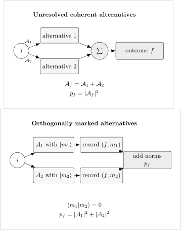
Coherent alternatives leading to one unresolved outcome are summed before taking the squared modulus. If orthogonal marker states preserve which-path information, the cross terms vanish and the corresponding probabilities add.

The state-based account of relative phase is in Superposition and Relative Phase. Physical two-slit realizations are treated in the Double-Slit Experiment, while environment-induced loss of local interference belongs to What Is Decoherence?.

Worked Example: Two Output Ports

Consider the normalized two-path state

$$\lvert\psi_\delta\rangle = \frac{ \lvert0\rangle + e^{i\delta}\lvert1\rangle }{\sqrt2}.$$

Let the output analyzer use

$$\lvert+\rangle = \frac{\lvert0\rangle+\lvert1\rangle}{\sqrt2}, \qquad \lvert-\rangle = \frac{\lvert0\rangle-\lvert1\rangle}{\sqrt2}.$$

The two output amplitudes are

$$\begin{aligned} \mathcal A_+ &= \langle+\rvert\psi_\delta\rangle = \frac{1+e^{i\delta}}{2}\\ &= e^{i\delta/2} \cos\frac{\delta}{2}, \end{aligned}$$

and

$$\begin{aligned} \mathcal A_- &= \langle-\rvert\psi_\delta\rangle = \frac{1-e^{i\delta}}{2}\\ &= -i e^{i\delta/2} \sin\frac{\delta}{2}. \end{aligned}$$

Therefore

$$p_+ = \cos^2\frac{\delta}{2}, \qquad p_- = \sin^2\frac{\delta}{2},$$

and $p_++p_-=1$. The common factor $e^{i\delta/2}$ affects neither probability. The relative phase $\delta$ matters because the analyzer recombines the path amplitudes.

Worked Example: A Qubit Analyzer

Write a normalized qubit as

$$\lvert\psi\rangle = \cos\frac{\theta}{2}\lvert0\rangle + e^{i\phi} \sin\frac{\theta}{2}\lvert1\rangle.$$

An equatorial analyzer state with phase $\gamma$ is

$$\lvert+_\gamma\rangle = \frac{ \lvert0\rangle + e^{i\gamma}\lvert1\rangle }{\sqrt2}.$$

The relevant amplitude is

$$\begin{aligned} \mathcal A(+_\gamma\leftarrow\psi) &= \frac{1}{\sqrt2} \left[ \cos\frac{\theta}{2} \right.\\ &\qquad\left. + e^{i(\phi-\gamma)} \sin\frac{\theta}{2} \right]. \end{aligned}$$

Its squared modulus is

$$p(+_\gamma) = \frac12 \left[ 1 + \sin\theta \cos(\phi-\gamma) \right].$$

This example separates three ingredients cleanly: the state amplitudes, the analyzer phase convention, and the final probability. Only the relative combination $\phi-\gamma$ appears in the prediction.

Intermediate Measurement Changes the Rule

The identity insertion used to compose amplitudes does not mean that an intermediate measurement occurred. Without such a measurement,

$$p_{\mathrm{unresolved}}(f) = \left\lvert \sum_n \langle f\rvert U_2\lvert n\rangle \langle n\rvert U_1\lvert i\rangle \right\rvert^2.$$

If a rank-one projective measurement of $n$ is actually performed and its outcome is ignored, the mutually exclusive joint probabilities add:

$$p_{\mathrm{measured}}(f) = \sum_n \left\lvert \langle f\rvert U_2\lvert n\rangle \langle n\rvert U_1\lvert i\rangle \right\rvert^2.$$

The two formulas differ by their cross terms. Inserting a mathematical resolution of the identity preserves coherence; performing a physical measurement generally does not. Projective state update is developed in Projective Measurement.

Phase Conventions and Invariant Predictions

If the source and target representatives are independently rephased,

$$\begin{aligned} \lvert\psi\rangle &\longmapsto e^{i\alpha}\lvert\psi\rangle,\\ \lvert\phi\rangle &\longmapsto e^{i\beta}\lvert\phi\rangle, \end{aligned}$$

then

$$\mathcal A(\phi\leftarrow\psi) \longmapsto e^{i(\alpha-\beta)} \mathcal A(\phi\leftarrow\psi).$$

The amplitude phase changes, but the transition probability does not.

An intermediate basis can also be rephased,

$$\lvert n\rangle \longmapsto e^{i\chi_n}\lvert n\rangle.$$

In each composed term,

$$\langle f\rvert U_2\lvert n\rangle \langle n\rvert U_1\lvert i\rangle,$$

the two factors acquire opposite phases and their product is unchanged. This is a useful audit: arbitrary phase conventions may change individual coordinates, but they must cancel from complete predictions.

The distinction among global phase, relative phase, and basis rephasing is developed in Rays and Global Phase.

Higher-Rank Outcomes

An outcome may correspond to a subspace rather than one ray. Let

$$P_a = \sum_{\alpha=1}^{d_a} \lvert a,\alpha\rangle \langle a,\alpha\rvert$$

project onto a $d_a$-dimensional eigenspace. The natural amplitude-level object is the branch vector

$$\lvert\psi_a\rangle = P_a\lvert\psi\rangle,$$

and its squared norm gives the outcome probability:

$$\begin{aligned} p(a) &= \lVert P_a\lvert\psi\rangle\rVert^2\\ &= \langle\psi\rvert P_a\lvert\psi\rangle\\ &= \sum_{\alpha=1}^{d_a} \lvert\langle a,\alpha\rvert\psi\rangle\rvert^2. \end{aligned}$$

The component amplitudes depend on the orthonormal basis chosen inside the eigenspace. Their squared sum does not. Calling any one of them the amplitude of the degenerate outcome would introduce an arbitrary basis choice.

This projector viewpoint is developed in Projectors and Projection-Valued Measures and applied in Born Rule for Discrete Spectra.

General Measurements and Mixed States

A general measurement can be described by measurement operators $M_{a\mu}$ satisfying

$$\sum_{a,\mu} M_{a\mu}^\dagger M_{a\mu} = I.$$

For a pure input, each refined branch has vector amplitude

$$\lvert\psi_{a\mu}\rangle = M_{a\mu}\lvert\psi\rangle.$$

If only the coarse outcome $a$ is recorded,

$$\begin{aligned} p(a) &= \sum_\mu \lVert M_{a\mu}\lvert\psi\rangle\rVert^2\\ &= \langle\psi\rvert E_a\lvert\psi\rangle, \end{aligned}$$

where

$$E_a = \sum_\mu M_{a\mu}^\dagger M_{a\mu}.$$

The POVM effect $E_a$ fixes the probability, but it does not uniquely fix the measurement operators or the post-measurement branches. Consequently, there is no unique scalar amplitude determined by $E_a$ alone. See POVMs: First Encounter for the general measurement language.

For a mixed state $\rho$, probabilities are

$$p(a) = \operatorname{Tr}(\rho E_a).$$

A mixed state generally has no unique state vector and therefore no unique list of pure-state amplitudes. Different ensemble decompositions of the same $\rho$ give the same operational probabilities. The canonical treatment is in Density Operators.

What Amplitudes Do and Do Not Mean

Probability amplitudes provide the linear bookkeeping from which quantum probabilities are computed. They encode:

• overlaps between prepared and tested rays;
• coordinates in a declared basis;
• coherent sums over unresolved alternatives;
• products along specified sequences;
• relative phases that can affect later interference.

They do not by themselves provide:

• a probability before the relevant modulus, norm, or trace rule is applied;
• a basis-independent phase for one isolated overlap;
• a classical probability distribution over every conceivable property;
• a unique scalar for a degenerate or general measurement outcome;
• an explanation of why nature uses the Born rule.

The probability postulate is the canonical subject of the Born Rule. Interpretive questions and proposed derivations belong to Foundations and Interpretations, which also develops the Bell, contextuality, and no-broadcasting no-go constraints. Those questions are distinct from the amplitude rules used here.

A Reliable Calculation Workflow

1. Name the preparation. Normalize the state or density operator.
2. Name the outcome structure. Use a ray, projector, or POVM effect that represents the actual measurement.
3. Include intervening evolution. Put the unitary or channel between preparation and measurement.
4. Decide whether alternatives are coherent. Sum amplitudes only when no physical record distinguishes the alternatives at the relevant stage.
5. Apply the correct probability rule. Take a squared modulus for a scalar amplitude, a squared norm for a branch vector, or a trace for a general state and effect.
6. Check completeness. Probabilities for an exhaustive measurement must sum or integrate to one.
7. Check invariance and units. Arbitrary basis phases must cancel, and continuous densities must carry the units required by their measure.

Diagnostic Checks

A trustworthy amplitude calculation should pass several quick tests.

Bounds. For normalized rays,

$$0 \leq \lvert\langle\phi\rvert\psi\rangle\rvert^2 \leq 1.$$

Completeness. For a complete orthonormal basis,

$$\sum_n \lvert\langle n\rvert\psi\rangle\rvert^2 = 1.$$

Rephasing. Replacing any basis ket by $e^{i\chi_n}\lvert n\rangle$ may change component phases but not the final probability.

Limiting phase. Equal two-path amplitudes should add maximally in phase and cancel when their relative phase is $\pi$.

Distinguishability. Orthogonal marker states should remove cross terms from the reduced detection probability.

Dimensions. A discrete amplitude is dimensionless for normalized kets; a continuous-label amplitude has inverse-square-root units of its measure.

Common Mistakes

• Treating an amplitude as though it were already a probability.
• Computing $\mathcal A^2$ instead of $\lvert\mathcal A\rvert^2=\mathcal A^*\mathcal A$.
• Adding probabilities for alternatives that remain coherent and unresolved.
• Adding amplitudes for outcomes that leave orthogonal physical records.
• Reading coefficients in one basis as probabilities for a different measurement basis.
• Assuming squared overlaps with nonorthogonal vectors must sum to one.
• Treating $\lvert\psi(x)\rvert^2$ as the probability of one exact continuous value rather than a density relative to $dx$.
• Assigning a unique scalar amplitude to a degenerate projector or POVM effect.
• Confusing insertion of a resolution of the identity with performance of an intermediate measurement.
• Attributing physical significance to the arbitrary phase of one isolated amplitude.

Canonical Boundaries and Cross-Links

• Born Rule owns the general probability postulate for projectors, density operators, continuous observables, and POVMs.
• Superposition and Relative Phase owns the state-level theory of coherent superpositions and relative phase.
• Transition Probabilities owns static and time-dependent transition calculations.
• Bases and Representations owns the general coordinate interpretation of ket components.
• Wavefunctions as Representations owns the systematic translation between abstract states and amplitude functions.
• Projective Measurement and POVMs: First Encounter own measurement update and general measurement structure.

References

• P. Busch, P. J. Lahti, J.-P. Pellonpää, and K. Ylinen, Quantum Measurement, Springer, 2016. Provides the modern effect, POVM, and instrument framework behind the general-measurement distinctions used here.
• P. A. M. Dirac, The Principles of Quantum Mechanics, 4th ed., Oxford University Press, 1958. The bra-ket and transformation-function viewpoint is foundational for amplitude language.
• R. P. Feynman, R. B. Leighton, and M. Sands, The Feynman Lectures on Physics, Vol. III, Chapter 3, Addison-Wesley, 1965. Develops the operational rules for adding and multiplying amplitudes.
• M. A. Nielsen and I. L. Chuang, Quantum Computation and Quantum Information, 10th anniversary ed., Cambridge University Press, 2010. Gives a concise finite-dimensional account of amplitudes, projective measurement, and general measurements.
• A. Peres, Quantum Theory: Concepts and Methods, Kluwer, 1995. Emphasizes the distinction between state descriptions, measurement outcomes, and operational probabilities.
• J. J. Sakurai and J. Napolitano, Modern Quantum Mechanics, 3rd ed., Cambridge University Press, 2020. See the opening treatment of state vectors, measurements, and basis amplitudes.

Exercises

Exercise 1: Order and complex conjugation

Let

$$\lvert\psi\rangle = \frac{\lvert0\rangle+i\lvert1\rangle}{\sqrt2}, \qquad \lvert\phi\rangle = \frac{\lvert0\rangle+\lvert1\rangle}{\sqrt2}.$$

Compute $\mathcal A(\phi\leftarrow\psi)$, $\mathcal A(\psi\leftarrow\phi)$, and their transition probabilities.

Solution

Taking the appropriate inner products,

$$\begin{aligned} \mathcal A(\phi\leftarrow\psi) &= \langle\phi\rvert\psi\rangle = \frac{1+i}{2},\\ \mathcal A(\psi\leftarrow\phi) &= \langle\psi\rvert\phi\rangle = \frac{1-i}{2}. \end{aligned}$$

They are complex conjugates. Both squared moduli are

$$\frac{ \lvert1+i\rvert^2 }{4} = \frac12.$$

The probabilities agree even though the ordered amplitudes are different.

Exercise 2: Basis amplitudes and completeness

In an orthonormal three-state basis, let

$$\lvert\psi\rangle = \frac{ 2\lvert0\rangle -i\lvert1\rangle +2\lvert2\rangle }{3}.$$

Find the three measurement amplitudes and verify normalization.

Solution

The amplitudes are the basis coefficients:

$$c_0=\frac23, \qquad c_1=-\frac{i}{3}, \qquad c_2=\frac23.$$

Their probabilities are

$$p_0=\frac49, \qquad p_1=\frac19, \qquad p_2=\frac49.$$

They satisfy

$$p_0+p_1+p_2 = \frac49+\frac19+\frac49 = 1.$$

Exercise 3: Two coherent paths

Two unresolved alternatives contribute

$$\mathcal A_1=\frac12, \qquad \mathcal A_2=\frac{e^{i\delta}}{2}$$

to one detector outcome. Find the probability and identify the phases of maximum and minimum probability.

Solution

Add the amplitudes before taking the squared modulus:

$$\begin{aligned} p &= \left\lvert \frac{1+e^{i\delta}}{2} \right\rvert^2\\ &= \cos^2\frac{\delta}{2}. \end{aligned}$$

The probability is maximal, $p=1$, when $\delta=2\pi k$. It vanishes when $\delta=(2k+1)\pi$, where the two amplitudes cancel.

Exercise 4: Partial distinguishability

Use the amplitudes from Exercise 3, but correlate the alternatives with marker states satisfying

$$\gamma = \langle m_1\rvert m_2\rangle.$$

Show that the detector probability is

$$p = \frac12 \left[ 1+\operatorname{Re} \left(\gamma e^{i\delta}\right) \right].$$

Interpret the cases $\gamma=1$ and $\gamma=0$.

Solution

The marked branch has squared norm

$$\begin{aligned} p &= \lvert\mathcal A_1\rvert^2 + \lvert\mathcal A_2\rvert^2\\ &\quad+ 2\operatorname{Re} \left( \mathcal A_1^*\mathcal A_2\gamma \right). \end{aligned}$$

Substituting the two amplitudes gives

$$p = \frac14+\frac14 + \frac12 \operatorname{Re} \left(\gamma e^{i\delta}\right),$$

which is the stated result. For $\gamma=1$, the marker states are identical and $p=\cos^2(\delta/2)$. For $\gamma=0$, they are orthogonal and $p=1/2$, independent of phase.

Exercise 5: Analyzer phase

For

$$\lvert\psi\rangle = \cos\frac{\theta}{2}\lvert0\rangle + e^{i\phi} \sin\frac{\theta}{2}\lvert1\rangle$$

and

$$\lvert+_\gamma\rangle = \frac{ \lvert0\rangle + e^{i\gamma}\lvert1\rangle }{\sqrt2},$$

derive $p(+_\gamma)$ and evaluate it for $\theta=\pi/2$ and $\gamma=\phi$.

Solution

The analyzer bra is

$$\langle+_\gamma\rvert = \frac{ \langle0\rvert + e^{-i\gamma}\langle1\rvert }{\sqrt2}.$$

Therefore

$$\begin{aligned} \mathcal A(+_\gamma\leftarrow\psi) &= \frac{1}{\sqrt2} \left[ \cos\frac{\theta}{2} \right.\\ &\qquad\left. + e^{i(\phi-\gamma)} \sin\frac{\theta}{2} \right]. \end{aligned}$$

Taking the squared modulus gives

$$p(+_\gamma) = \frac12 \left[ 1+\sin\theta\cos(\phi-\gamma) \right].$$

For $\theta=\pi/2$ and $\gamma=\phi$, the state equals the analyzer ray up to phase convention, and $p(+_\gamma)=1$.

Exercise 6: Degenerate outcome

Let

$$P = \lvert1\rangle\langle1\rvert + \lvert2\rangle\langle2\rvert$$

and

$$\lvert\psi\rangle = c_0\lvert0\rangle +c_1\lvert1\rangle +c_2\lvert2\rangle.$$

Find the probability of the outcome $P$. Explain why a unitary change of basis inside $\operatorname{ran}P$ cannot change it.

Solution

The projected branch is

$$P\lvert\psi\rangle = c_1\lvert1\rangle + c_2\lvert2\rangle,$$

so

$$p(P) = \lVert P\lvert\psi\rangle\rVert^2 = \lvert c_1\rvert^2+\lvert c_2\rvert^2.$$

Any other orthonormal basis $\{\lvert u\rangle,\lvert v\rangle\}$ of the same subspace is related by a two-dimensional unitary matrix. Unitarity preserves the component norm:

$$\lvert\langle u\rvert\psi\rangle\rvert^2 + \lvert\langle v\rvert\psi\rangle\rvert^2 = \lvert c_1\rvert^2+\lvert c_2\rvert^2.$$

The scalar components depend on the internal basis; the projector probability does not.

Exercise 7: Continuous-amplitude units

Suppose $x$ has dimensions of length and

$$\int_{\mathbb R} \lvert\psi_x(x)\rvert^2\,dx = 1.$$

Define the dimensionless coordinate $q=x/L$ for a fixed length $L$. Find a normalized amplitude $\psi_q(q)$ and state the units of $\psi_x$.

Solution

Since $x=Lq$, one has $dx=L\,dq$. Probability preservation requires

$$\lvert\psi_q(q)\rvert^2\,dq = \lvert\psi_x(Lq)\rvert^2L\,dq.$$

One convenient phase convention is therefore

$$\psi_q(q) = \sqrt L\,\psi_x(Lq).$$

Indeed,

$$\int \lvert\psi_q(q)\rvert^2\,dq = \int \lvert\psi_x(x)\rvert^2\,dx = 1.$$

Because $dx$ has units $L$, the original amplitude has units $[\psi_x]=L^{-1/2}$. The dimensionless-coordinate amplitude $\psi_q$ is dimensionless.

Exercise 8: Identity insertion or actual measurement?

Two intermediate alternatives have amplitudes

$$a_0=a_1=\frac{1}{\sqrt2}$$

from the source, followed by

$$b_0=\frac{1}{\sqrt2}, \qquad b_1=-\frac{1}{\sqrt2}$$

to a selected final outcome. Compare the final probability when the intermediate alternative is unresolved with the probability when it is measured and the result is ignored.

Solution

Without an intermediate measurement, the alternatives are coherent:

$$\mathcal A = b_0a_0+b_1a_1 = \frac12-\frac12 = 0.$$

Hence $p_{\mathrm{unresolved}}=0$.

If the intermediate alternative is measured, the mutually exclusive joint probabilities add:

$$\begin{aligned} p_{\mathrm{measured}} &= \lvert b_0a_0\rvert^2 + \lvert b_1a_1\rvert^2\\ &= \frac14+\frac14 = \frac12. \end{aligned}$$

The measurement removes the cross term that produced destructive interference.