Probability in Different Bases

To predict a projective measurement, express the state in the eigenspaces selected by that measurement and then apply the Born rule. If a normalized state is expanded in a nondegenerate measurement basis as

$$|\psi\rangle = \sum_a d_a|f_a\rangle,$$

then

$$p(a) = |d_a|^2 = |\langle f_a|\psi\rangle|^2.$$

The same abstract state has different component lists in different bases. Those lists are coordinate descriptions, while choosing a different measurement basis is a different physical question. Keeping that distinction clear prevents most basis-probability mistakes.

This page owns the probability workflow and its standard spin, qubit, and energy-basis applications. The abstract transformation algebra is canonical at Change of Basis, and measurement conditioning after an outcome belongs at Measurement in a Chosen Basis.

Required background. Probability Amplitudes supplies basis coefficients as amplitudes; Born Rule for Discrete Spectra supplies discrete measurement probabilities.

Helpful background. Change of Basis supplies the unitary overlap matrix between coordinate systems.

The measurement determines the relevant components

Let $A$ be a nondegenerate observable with eigenvectors $|f_a\rangle$:

$$A|f_a\rangle = a|f_a\rangle.$$

Its spectral projectors are

$$P_a = |f_a\rangle\langle f_a|.$$

The Born probability is

$$\begin{aligned} p(a) &= \langle\psi|P_a|\psi\rangle\\ &= |\langle f_a|\psi\rangle|^2. \end{aligned}$$

The coefficient to square is therefore the overlap with the measurement eigenvector, not necessarily a coefficient in the basis in which the state happened to be supplied.

Overlap matrix between two bases

Suppose the state is known in an orthonormal source basis $\{|e_n\rangle\}$:

$$|\psi\rangle = \sum_n c_n|e_n\rangle, \qquad c_n=\langle e_n|\psi\rangle.$$

Let $\{|f_a\rangle\}$ be the measurement basis and define the overlap matrix

$$S_{an} \equiv \langle f_a|e_n\rangle.$$

The measurement-basis amplitudes are

$$\begin{aligned} d_a &= \langle f_a|\psi\rangle\\ &= \sum_nS_{an}c_n. \end{aligned}$$

In column-vector notation,

$$\mathbf d=S\mathbf c.$$

The probabilities are computed only after this amplitude transformation:

$$p(a)=|d_a|^2.$$

Why the overlap matrix is unitary

Completeness of the source basis gives

$$\begin{aligned} (SS^\dagger)_{ab} &= \sum_n \langle f_a|e_n\rangle \langle e_n|f_b\rangle\\ &= \langle f_a|f_b\rangle = \delta_{ab}. \end{aligned}$$

Similarly, $S^\dagger S=I$. Thus

$$S^\dagger=S^{-1}.$$

Unitarity preserves normalization:

$$\begin{aligned} \sum_a|d_a|^2 &= \mathbf d^\dagger\mathbf d\\ &= \mathbf c^\dagger S^\dagger S\mathbf c\\ &= \mathbf c^\dagger\mathbf c =1. \end{aligned}$$

Failure of the transformed probabilities to sum to one is therefore a sign of an inconsistent basis convention, a nonunitary overlap matrix, truncation, or an unnormalized state.

Probability workflow

The practical sequence is short:

1. Identify the measurement projectors or eigenbasis.
2. Compute overlaps between that basis and the basis in which the state is known.
3. Transform amplitudes, including their complex phases.
4. Take squared moduli or apply the relevant subspace projector.
5. Check positivity and normalization.

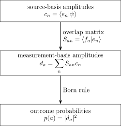
Amplitudes, not probabilities, transform linearly. The unitary overlap matrix $S_{an}=\langle f_a|e_n\rangle$ produces measurement-basis amplitudes $\mathbf d=S\mathbf c$; the Born rule is applied only at the final step.

For a degenerate measurement, replace the basis-vector step by the projector onto the complete eigenspace.

Passive coordinates versus a new measurement

A passive basis change rewrites the same state and the same physical projector in new coordinates. If

$$\mathbf d=S\mathbf c$$

and the projector matrices obey

$$P_f = SP_eS^\dagger,$$

then

$$\begin{aligned} \mathbf d^\dagger P_f\mathbf d &= \mathbf c^\dagger S^\dagger SP_eS^\dagger S \mathbf c\\ &= \mathbf c^\dagger P_e\mathbf c. \end{aligned}$$

The prediction is unchanged because only the coordinates changed.

Choosing a different measurement basis holds the prepared state fixed and changes the projectors being tested. Measuring $S_z$ and measuring $S_x$ are different physical procedures and can produce different probability distributions.

Active unitary transformations

Applying a unitary $V$ to the state while keeping the measurement fixed is an active operation:

$$|\psi\rangle \mapsto V|\psi\rangle.$$

The probability becomes

$$\begin{aligned} p'_a &= \langle\psi|V^\dagger P_aV|\psi\rangle\\ &= |\langle f_a|V|\psi\rangle|^2. \end{aligned}$$

This can be calculated by transforming the state forward or the projector backward, but it is not a passive rewrite. The physical preparation or measurement apparatus has changed.

Why old probabilities are not enough

For a coherent pure state,

$$d_a = \sum_nS_{an}c_n.$$

Squaring gives

$$\begin{aligned} p(a) &= \sum_n|S_{an}|^2|c_n|^2\\ &\quad+ \sum_{n\ne m} S_{an}S_{am}^*c_nc_m^*. \end{aligned}$$

The second line contains interference terms and depends on relative phases. Therefore one generally cannot transform old-basis probabilities $|c_n|^2$ into new-basis probabilities without retaining the amplitudes or the full density operator.

When a stochastic probability map is valid

If the state is incoherent and diagonal in the source basis,

$$\rho = \sum_np_n|e_n\rangle\langle e_n|,$$

then the measurement probabilities are

$$q_a = \sum_n|S_{an}|^2p_n.$$

For finite discrete orthonormal bases, the matrix

$$B_{an}=|S_{an}|^2$$

is doubly stochastic. The same statement extends to countable discrete bases when the sums converge. In this special case it maps the classical population vector $\mathbf p$ to $\mathbf q$. For a coherent state with off-diagonal matrix elements in the source basis, this population-only rule omits physical interference.

Density operators in the measurement basis

Let $\rho_e$ be the density matrix in the source basis. In the measurement basis,

$$\rho_f = S\rho_eS^\dagger.$$

For a rank-one basis measurement,

$$p(a) = (\rho_f)_{aa}.$$

Off-diagonal coherences in $\rho_e$ can contribute to diagonal populations in $\rho_f$. This is the mixed-state version of relative-phase interference.

The matrix entries are basis dependent, while the scalar Born probability

$$p(a) = \operatorname{Tr}(\rho P_a)$$

is representation independent when both $\rho$ and $P_a$ describe the same physical objects.

Degenerate measurements

If outcome $a$ has eigenspace projector $P_a$ with rank greater than one, the probability is

$$p(a) = \langle\psi|P_a|\psi\rangle.$$

For any orthonormal basis $\{|a,r\rangle\}$ of that eigenspace,

$$p(a) = \sum_r|\langle a,r|\psi\rangle|^2.$$

Changing basis inside the degenerate eigenspace cannot change the coarse outcome probability. Treating each arbitrarily chosen basis vector as a separate physical outcome would add a refinement not specified by the original observable.

Generalized measurements need not select a basis

Not every measurement is an orthonormal-basis measurement. A POVM assigns effects $E_y$ satisfying

$$E_y\ge0, \qquad \sum_yE_y=I,$$

with probabilities

$$p(y)=\operatorname{Tr}(\rho E_y).$$

The “express the state in the measurement basis” shortcut applies to rank-one projective measurements. The effect form is the reliable general rule.

Spin prepared along z and measured along x

For spin one-half,

$$|\pm x\rangle = \frac{|+z\rangle\pm|-z\rangle}{\sqrt2}.$$

Inverting gives

$$|+z\rangle = \frac{|+x\rangle+|-x\rangle}{\sqrt2}.$$

Thus an $S_x$ measurement on $|+z\rangle$ gives

$$p(+x)=\frac12, \qquad p(-x)=\frac12.$$

The state is sharp in the $z$ basis and unbiased in the $x$ basis. This is a change of physical measurement, not a claim that the state has become mixed.

Spin along an arbitrary axis

Let the unit vector $\mathbf n$ have polar angles $(\theta,\phi)$. A convenient eigenbasis of $\mathbf n\cdot\boldsymbol\sigma$ is

$$\begin{aligned} |+\mathbf n\rangle &= \cos\frac\theta2|+z\rangle + e^{i\phi}\sin\frac\theta2|-z\rangle,\\ |-\mathbf n\rangle &= -e^{-i\phi}\sin\frac\theta2|+z\rangle + \cos\frac\theta2|-z\rangle. \end{aligned}$$

For a system prepared in $|+z\rangle$,

$$\begin{aligned} p(+\mathbf n) &= \cos^2\frac\theta2,\\ p(-\mathbf n) &= \sin^2\frac\theta2. \end{aligned}$$

Only the angle between preparation and measurement axes matters for these probabilities.

Computational and Hadamard bases

Let

$$|\psi\rangle = \frac{\sqrt3}{2}|0\rangle + \frac12|1\rangle.$$

In the computational basis,

$$p(0)=\frac34, \qquad p(1)=\frac14.$$

The Hadamard basis is

$$|\pm\rangle = \frac{|0\rangle\pm|1\rangle}{\sqrt2}.$$

The amplitudes are

$$\begin{aligned} d_+ &= \frac{\sqrt3+1}{2\sqrt2},\\ d_- &= \frac{\sqrt3-1}{2\sqrt2}. \end{aligned}$$

Therefore

$$p(+) = \frac{2+\sqrt3}{4}, \qquad p(-) = \frac{2-\sqrt3}{4}.$$

The distributions differ because the two measurements ask different questions of the same state.

Relative phase becomes probability

For

$$|\psi\rangle = \alpha|0\rangle+\beta|1\rangle, \qquad |\alpha|^2+|\beta|^2=1,$$

the Hadamard amplitudes are

$$d_\pm = \frac{\alpha\pm\beta}{\sqrt2}.$$

Hence

$$\begin{aligned} p(+) &= \frac12+ \operatorname{Re}(\alpha^*\beta),\\ p(-) &= \frac12- \operatorname{Re}(\alpha^*\beta). \end{aligned}$$

The computational-basis probabilities know only $|\alpha|^2$ and $|\beta|^2$. The Hadamard measurement converts one quadrature of the relative coherence $\alpha^*\beta$ into an observable population difference. This is why Superposition and Relative Phase has operational content.

Mutually unbiased bases

Two orthonormal bases are mutually unbiased if

$$|\langle f_a|e_n\rangle|^2 = \frac1d$$

for every $a,n$ in dimension $d$. Preparing any source-basis vector $|e_n\rangle$ then gives the uniform distribution

$$p(a)=\frac1d$$

in the other basis. The computational and Hadamard bases are mutually unbiased for a qubit. Mutually unbiased does not mean that every superposition gives a uniform distribution; interference among several source amplitudes can still produce structure.

Energy-basis measurements

Let a Hamiltonian have nondegenerate eigenstates $|E_n\rangle$. If

$$|\psi\rangle = \sum_nc_n|E_n\rangle,$$

then

$$p(E_n)=|c_n|^2.$$

For the oscillator superposition

$$|\psi\rangle = \sqrt{\frac35}|E_0\rangle + e^{i\alpha}\sqrt{\frac25}|E_2\rangle,$$

an energy measurement gives

$$p(E_0)=\frac35, \qquad p(E_2)=\frac25.$$

The phase $e^{i\alpha}$ is invisible in this basis because the energy projectors are diagonal. It can affect a measurement in another basis.

From a wavefunction to energy amplitudes

If the state is supplied as $\psi(x)=\langle x|\psi\rangle$ and the normalized energy eigenfunctions are

$$\psi_n(x)=\langle x|E_n\rangle,$$

then

$$\begin{aligned} c_n &= \langle E_n|\psi\rangle\\ &= \int_{-\infty}^{\infty} \psi_n(x)^*\psi(x)\,dx. \end{aligned}$$

The overlap integral is the change from position amplitudes to energy amplitudes. After computing all relevant $c_n$, the energy probabilities are $|c_n|^2$. Degenerate and continuous sectors require spectral projectors and the appropriate measures.

Continuous measurement bases

In a generalized continuous basis $|\lambda\rangle$, the transformed amplitude is an integral transform:

$$\psi_f(\lambda) = \int dx\, \langle\lambda|x\rangle\psi(x).$$

With delta-normalization relative to $d\lambda$, the probability density is

$$p_f(\lambda) = |\psi_f(\lambda)|^2,$$

and interval probabilities are integrals of this density. The kernel, normalization factors, and integration measure are part of the basis convention. For position–momentum Fourier conventions, see Operator Representations and Born Rule for Continuous Spectra.

What multiple bases reveal

A single basis measurement determines only the diagonal populations in that basis. Measurements in additional bases can reveal coherence that was hidden in those populations. This is the elementary reason state tomography requires more than one measurement setting.

It does not follow that the state possessed simultaneous definite values in all those bases. Each basis specifies a different measurement context, and probabilities must be computed for that context.

Practical checks

Before trusting a basis-probability calculation, check:

• The source and measurement bases are orthonormal and use consistent phases.
• The overlap matrix convention matches $S_{an}=\langle f_a|e_n\rangle$.
• $S^\dagger S=I$ to the intended numerical precision.
• Amplitudes, including phases, were transformed before taking moduli.
• Degenerate outcomes were represented by full eigenspace projectors.
• The final probabilities are real, nonnegative, and sum to one.
• State vectors, operators, and projectors were not mixed across coordinate conventions.

Superposition language

Whether a state is “a superposition” is basis dependent. Every normalized vector is a basis vector in some orthonormal basis and a multi-term superposition in many others.

The invariant statement is operational:

A state and a specified measurement determine a Born probability distribution.

Basis labels describe how the calculation is organized. The projectors or effects identify the physical measurement.

Common mistakes

Squaring coefficients in the wrong basis

Coefficients in the preparation basis are not automatically probabilities for a different measurement. Project onto the measurement eigenspaces first.

Transforming probabilities instead of amplitudes

Relative phases create interference terms. A stochastic map built from $|S_{an}|^2$ applies to source-basis populations only when the state is incoherent in that basis.

Confusing passive and active changes

Changing coordinates for both state and projector leaves predictions unchanged. Rotating the state or changing the measurement projectors is a physical operation.

Losing complex conjugation

$S_{an}=\langle f_a|e_n\rangle$ is not generally equal to $\langle e_n|f_a\rangle$; the two are complex conjugates.

Refining a degenerate outcome accidentally

A basis chosen inside a degenerate eigenspace is not unique. Sum over that subspace unless an additional commuting measurement resolves it.

Ignoring continuous-basis measures

Generalized basis amplitudes are densities relative to a convention. Include the correct integration measure and normalization factors.

Summary

If $\mathbf c$ contains state amplitudes in a source basis and

$$S_{an}=\langle f_a|e_n\rangle,$$

then measurement-basis amplitudes are

$$\mathbf d=S\mathbf c,$$

and rank-one projective probabilities are

$$p(a)=|d_a|^2.$$

The overlap matrix is unitary, so normalization is preserved. Passive coordinate changes leave Born scalars invariant; choosing a new measurement basis changes the physical projectors. Relative phase can become population in the new basis, which is why amplitudes or the full density operator must be transformed before probabilities are extracted.

References

• P. A. M. Dirac, The Principles of Quantum Mechanics, 4th ed., Oxford University Press, 1958, Chapters II–III.
• D. J. Griffiths and D. F. Schroeter, Introduction to Quantum Mechanics, 3rd ed., Cambridge University Press, 2018, Chapters 3–4.
• M. A. Nielsen and I. L. Chuang, Quantum Computation and Quantum Information, 10th anniversary ed., Cambridge University Press, 2010, Chapters 2 and 4.
• J. J. Sakurai and J. Napolitano, Modern Quantum Mechanics, 3rd ed., Cambridge University Press, 2020, Chapters 1–2.
• R. Shankar, Principles of Quantum Mechanics, 2nd ed., Springer, 1994, Chapters 1 and 4.
• J. von Neumann, Mathematical Foundations of Quantum Mechanics, Princeton University Press, 1955, Chapters II–III.

Exercises

1. Spin from z to x

A spin-one-half system is prepared in $|+z\rangle$. Compute the probabilities of $S_x=+\hbar/2$ and $S_x=-\hbar/2$.

Solution

Use

$$|+z\rangle = \frac{|+x\rangle+|-x\rangle}{\sqrt2}.$$

Both measurement-basis amplitudes have modulus $1/\sqrt2$, so

$$p(+x)=\frac12, \qquad p(-x)=\frac12.$$

2. Relative phase in the Hadamard basis

Let

$$|\psi_\phi\rangle = \frac{|0\rangle+e^{i\phi}|1\rangle}{\sqrt2}.$$

Find the probabilities in the Hadamard basis.

Solution

The amplitudes are

$$d_\pm = \frac{1\pm e^{i\phi}}{2}.$$

Therefore

$$\begin{aligned} p(+) &= \frac{1+\cos\phi}{2},\\ p(-) &= \frac{1-\cos\phi}{2}. \end{aligned}$$

The computational-basis probabilities are always $1/2$, but the Hadamard probabilities reveal the relative phase quadrature $\cos\phi$.

3. Oscillator energy measurement

For

$$|\psi\rangle = \sqrt{\frac35}|E_0\rangle + e^{i\alpha}\sqrt{\frac25}|E_2\rangle,$$

find the energy probabilities and explain the role of $\alpha$.

Solution

The state is already in the nondegenerate energy basis, so

$$p(E_0)=\frac35, \qquad p(E_2)=\frac25,$$

with every other energy probability zero. The phase $\alpha$ is invisible to this diagonal measurement but can affect probabilities in a basis that mixes $|E_0\rangle$ and $|E_2\rangle$.

4. A phase-dependent two-level transformation

Let

$$\mathbf c = \begin{pmatrix} \sqrt3/2\\ e^{i\phi}/2 \end{pmatrix}, \qquad S = \frac1{\sqrt2} \begin{pmatrix} 1&1\\ 1&-1 \end{pmatrix}.$$

Compute the two measurement probabilities.

Solution

The transformed amplitudes are

$$\mathbf d = \frac1{2\sqrt2} \begin{pmatrix} \sqrt3+e^{i\phi}\\ \sqrt3-e^{i\phi} \end{pmatrix}.$$

Taking squared moduli gives

$$\begin{aligned} p_1 &= \frac12+\frac{\sqrt3}{4}\cos\phi,\\ p_2 &= \frac12-\frac{\sqrt3}{4}\cos\phi. \end{aligned}$$

The probabilities sum to one and remain nonnegative for every $\phi$.

5. Passive invariance

Suppose $\mathbf d=S\mathbf c$ and $P_f=SP_eS^\dagger$ with unitary $S$. Prove that the Born probability is unchanged.

Solution

Substitute both transformation laws:

$$\begin{aligned} \mathbf d^\dagger P_f\mathbf d &= \mathbf c^\dagger S^\dagger (SP_eS^\dagger)S\mathbf c\\ &= \mathbf c^\dagger P_e\mathbf c, \end{aligned}$$

because $S^\dagger S=I$. State and projector coordinates changed together, so the physical scalar did not.

6. Coherence becomes a population difference

In the computational basis, let

$$\rho = \begin{pmatrix} 1/2 & z\\ z^* & 1/2 \end{pmatrix}.$$

Find the Hadamard-basis probabilities. Which part of $z$ do they reveal?

Solution

Using $p(\pm)=\langle\pm|\rho|\pm\rangle$,

$$\begin{aligned} p(+) &= \frac12+\operatorname{Re}z,\\ p(-) &= \frac12-\operatorname{Re}z. \end{aligned}$$

The computational populations are both $1/2$, while the Hadamard population difference is $2\operatorname{Re}z$. A different phase-sensitive basis is needed to reveal $\operatorname{Im}z$.

7. Mutually unbiased bases

Suppose $|\langle f_a|e_n\rangle|^2=1/d$ for every $a,n$. Show that a state prepared as any one $|e_n\rangle$ gives a uniform $f$-basis distribution.

Solution

For the preparation $|e_n\rangle$, the $f$-basis amplitude is

$$d_a=\langle f_a|e_n\rangle.$$

Therefore

$$p(a)=|d_a|^2=\frac1d$$

for every $a$. Summing over the $d$ outcomes gives one.

8. Degenerate energy outcome

An energy $E$ has orthonormal degenerate eigenvectors $|E,1\rangle$ and $|E,2\rangle$. A normalized state has amplitudes $c_1$ and $c_2$ in those directions, plus components orthogonal to the eigenspace. Find the probability of measuring energy $E$ and show that it is unchanged by a unitary basis change within the eigenspace.

Solution

The energy projector is

$$P_E = |E,1\rangle\langle E,1| + |E,2\rangle\langle E,2|.$$

Hence

$$p(E)=|c_1|^2+|c_2|^2.$$

A unitary transformation within the two-dimensional eigenspace preserves the norm of the coefficient vector $(c_1,c_2)^{\mathsf T}$, so the sum and the coarse energy probability are unchanged.