Change of Basis

A change of basis rewrites the same quantum state, operator, and measurement in a different coordinate system. It changes component columns and matrix entries, but it does not change the abstract objects or any physical prediction when every represented object is transformed consistently.

This distinction is easy to state and unusually easy to mishandle. A unitary matrix can describe a passive coordinate rewrite, an active physical operation, or a change in which observable an apparatus measures. Those three uses share algebra but answer different physical questions.

This page fixes one passive convention and uses it throughout. The general linear-algebra theory of arbitrary invertible coordinate changes belongs to Change of Basis in the Mathematical Toolkit. Here the emphasis is quantum-mechanical bookkeeping: amplitudes, observables, density operators, continuous representations, composite systems, and basis-independent checks.

Convention at a Glance

Let

$$\mathcal E=\{\lvert e_n\rangle\}, \qquad \mathcal F=\{\lvert f_a\rangle\}$$

be two ordered orthonormal bases of the same Hilbert space. Define the overlap matrix with new-basis labels on rows and old-basis labels on columns:

$$S_{an}=\langle f_a\vert e_n\rangle.$$

If $c$ is the old component column and $d$ is the new component column, then

$$d=Sc.$$

The matching operator rule is

$$A_{\mathcal F}=S A_{\mathcal E}S^\dagger.$$

These two equations must travel together. They determine every convention on this page.

Object	Passive transformation rule
State components	$d=Sc$
Basis ket	$\lvert f_a\rangle=\sum_n S_{an}^*\lvert e_n\rangle$
Operator	$A_{\mathcal F}=S A_{\mathcal E}S^\dagger$
Density operator	$\rho_{\mathcal F}=S\rho_{\mathcal E}S^\dagger$
Measurement effect	$(E_r)_{\mathcal F}=S(E_r)_{\mathcal E}S^\dagger$

Some books define their basis-change matrix as $S^\dagger$, so their formulas place daggers on the opposite side. Neither convention is intrinsically better. A reliable calculation labels the matrix entries, derives one component formula, and then remains consistent.

The Abstract Object and Its Representatives

A ket is not a column of numbers until a basis has been chosen. The coordinate maps associated with $\mathcal E$ and $\mathcal F$ send the same abstract ket to two different columns:

$$R_{\mathcal E}\lvert\psi\rangle=c, \qquad R_{\mathcal F}\lvert\psi\rangle=d.$$

The overlap matrix is the coordinate map between those representations:

$$S=R_{\mathcal F}R_{\mathcal E}^{-1}, \qquad d=Sc.$$

Likewise, one abstract operator has different matrices,

$$A_{\mathcal E} = R_{\mathcal E}A R_{\mathcal E}^{-1}, \qquad A_{\mathcal F} = R_{\mathcal F}A R_{\mathcal F}^{-1}.$$

The following diagram separates the objects from their representatives and shows where the invariant prediction lives.

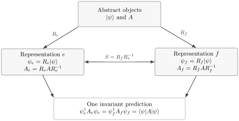
The coordinate maps $R_{\mathcal E}$ and $R_{\mathcal F}$ produce different columns and matrices. The overlap map $S$ connects the representations, while $\langle\psi\vert A\vert\psi\rangle$ is independent of either choice.

The distinction between an object and its representation is developed more broadly in Bases and Representations.

Why the Overlap Matrix Is Unitary

Because both bases are complete and orthonormal,

$$\sum_n \lvert e_n\rangle\langle e_n\rvert=I, \qquad \sum_a \lvert f_a\rangle\langle f_a\rvert=I.$$

The matrix product $SS^\dagger$ has entries

$$\begin{aligned} (SS^\dagger)_{ab} &= \sum_n S_{an}S_{bn}^* \\ &= \sum_n \langle f_a\vert e_n\rangle \langle e_n\vert f_b\rangle \\ &= \langle f_a\vert f_b\rangle \\ &= \delta_{ab}. \end{aligned}$$

Similarly,

$$\begin{aligned} (S^\dagger S)_{nm} &= \sum_a S_{an}^*S_{am} \\ &= \sum_a \langle e_n\vert f_a\rangle \langle f_a\vert e_m\rangle \\ &= \delta_{nm}. \end{aligned}$$

Therefore

$$SS^\dagger=S^\dagger S=I, \qquad S^{-1}=S^\dagger.$$

This is not an extra physical postulate. It follows from comparing two orthonormal coordinate systems on the same Hilbert space. For nonorthonormal bases, the coordinate map is generally invertible but not unitary.

Basis Kets and State Components Transform Oppositely

Insert the old completeness relation into a new basis ket:

$$\begin{aligned} \lvert f_a\rangle &= \sum_n \lvert e_n\rangle \langle e_n\vert f_a\rangle \\ &= \sum_n S_{an}^*\lvert e_n\rangle. \end{aligned}$$

The inverse relation is

$$\lvert e_n\rangle = \sum_a S_{an}\lvert f_a\rangle.$$

Now write the same state in both bases:

$$\lvert\psi\rangle = \sum_n c_n\lvert e_n\rangle = \sum_a d_a\lvert f_a\rangle.$$

Taking the overlap with $\langle f_a\rvert$ gives

$$\begin{aligned} d_a &= \langle f_a\vert\psi\rangle \\ &= \sum_n \langle f_a\vert e_n\rangle c_n \\ &= \sum_n S_{an}c_n. \end{aligned}$$

Thus basis kets carry $S^*$ in their old-basis expansion, while ket components carry $S$. This opposite motion is what leaves the abstract sum $\sum_n c_n\lvert e_n\rangle$ unchanged.

A Practical Dictionary for Matrix Conventions

Numerical linear algebra packages commonly return a matrix $V$ whose columns are the new basis vectors written in old coordinates:

$$V = \begin{pmatrix} [f_1]_{\mathcal E} & \cdots & [f_N]_{\mathcal E} \end{pmatrix}.$$

Its entries are

$$V_{na} = \langle e_n\vert f_a\rangle = S_{an}^*.$$

Therefore

$$V=S^\dagger, \qquad S=V^\dagger.$$

The equivalent formulas in the column-eigenvector convention are

$$c=Vd, \qquad d=V^\dagger c, \qquad A_{\mathcal F}=V^\dagger A_{\mathcal E}V.$$

This dictionary resolves most apparent conflicts between textbooks and software. Before using a memorized similarity transformation, ask what the columns of the matrix actually contain.

Composition and Reversal

Suppose $S_{\mathcal F\leftarrow\mathcal E}$ maps $\mathcal E$ components to $\mathcal F$ components, and $S_{\mathcal G\leftarrow\mathcal F}$ maps $\mathcal F$ components to $\mathcal G$ components. Then

$$S_{\mathcal G\leftarrow\mathcal E} = S_{\mathcal G\leftarrow\mathcal F} S_{\mathcal F\leftarrow\mathcal E}.$$

The rightmost conversion acts first. Reversing a conversion takes the adjoint:

$$S_{\mathcal E\leftarrow\mathcal F} = S_{\mathcal F\leftarrow\mathcal E}^\dagger.$$

These relations are useful diagnostics. A chain of exact orthonormal basis changes must remain unitary, and a round trip must return the identity.

State Norms and Inner Products

For two states with old columns $c$ and $b$, the new columns are

$$d=Sc, \qquad a=Sb.$$

Their inner product is unchanged:

$$a^\dagger d = b^\dagger S^\dagger S c = b^\dagger c.$$

In particular,

$$d^\dagger d=c^\dagger c.$$

Normalization is therefore representation-independent. A basis change cannot repair an unnormalized state or turn a nonzero state into the zero vector; it only redistributes the same norm among components. See Normalization for ordinary, continuum, box, and flux conventions.

Transition amplitudes also remain invariant when both endpoint states are rewritten consistently:

$$\langle\phi\vert\psi\rangle = b^\dagger c = (Sb)^\dagger(Sc).$$

Operator Matrices

Let

$$(A_{\mathcal E})_{mn} = \langle e_m\vert A\vert e_n\rangle.$$

In the new basis,

$$\begin{aligned} (A_{\mathcal F})_{ab} &= \langle f_a\vert A\vert f_b\rangle \\ &= \sum_{m,n} \langle f_a\vert e_m\rangle (A_{\mathcal E})_{mn} \langle e_n\vert f_b\rangle \\ &= \sum_{m,n} S_{am}(A_{\mathcal E})_{mn}S_{bn}^*. \end{aligned}$$

Hence

$$A_{\mathcal F} = S A_{\mathcal E}S^\dagger.$$

The identity operator remains the identity, but a general operator need not retain its pattern of entries. Diagonality, sparsity, band structure, and the size of individual matrix elements are representation-dependent.

The transformation respects operator algebra:

$$\begin{aligned} (AB)_{\mathcal F} &= A_{\mathcal F}B_{\mathcal F}, \\ [A,B]_{\mathcal F} &= S[A,B]_{\mathcal E}S^\dagger, \\ (A^\dagger)_{\mathcal F} &= (A_{\mathcal F})^\dagger. \end{aligned}$$

Consequently Hermiticity, unitarity, normality, commutation relations, and operator identities do not depend on the orthonormal basis used to display them. Other representation forms are catalogued in Operator Representations.

Expectation Values and Matrix Elements

Transform the state and operator together:

$$d=Sc, \qquad A_{\mathcal F}=S A_{\mathcal E}S^\dagger.$$

Then

$$\begin{aligned} d^\dagger A_{\mathcal F}d &= c^\dagger S^\dagger \left(SA_{\mathcal E}S^\dagger\right) Sc \\ &= c^\dagger A_{\mathcal E}c. \end{aligned}$$

The same cancellation proves invariance of a general matrix element:

$$(Sb)^\dagger \left(SA_{\mathcal E}S^\dagger\right) (Sc) = b^\dagger A_{\mathcal E}c.$$

If a calculation gives different expectation values in two bases, the physics has not become basis-dependent. At least one state, operator, index ordering, or conjugation was transformed inconsistently.

Spectra and Eigenvectors

Suppose an old-coordinate eigenvector $v$ satisfies

$$A_{\mathcal E}v=\lambda v.$$

Its new-coordinate column is $Sv$, and

$$\begin{aligned} A_{\mathcal F}(Sv) &= SA_{\mathcal E}S^\dagger Sv \\ &= S A_{\mathcal E}v \\ &= \lambda Sv. \end{aligned}$$

Thus eigenvalues and eigenspace dimensions are unchanged. In finite dimension, unitary similarity also preserves the characteristic polynomial, trace, determinant, rank, and singular values.

An individual eigenvector inside a degenerate eigenspace is not canonical. If $A$ has eigenvalue $\lambda$ on a subspace $\mathcal H_\lambda$, any orthonormal rotation within $\mathcal H_\lambda$ gives another valid eigenbasis. The invariant object is the spectral projector

$$P_\lambda = \sum_{a\in\lambda} \lvert f_a\rangle\langle f_a\rvert,$$

not the phase or orientation of each displayed eigenvector. This matters in analytic derivations and in numerical diagonalization near degeneracies.

Diagonalization as a Basis Choice

Let $A_{\mathcal E}$ be Hermitian, and let a unitary matrix $V$ contain an orthonormal eigenbasis in its columns:

$$A_{\mathcal E}V=V\Lambda, \qquad V^\dagger V=I.$$

The new basis consists of those eigenvectors. Since $S=V^\dagger$,

$$A_{\mathcal F} = V^\dagger A_{\mathcal E}V = \Lambda.$$

State components in the eigenbasis are

$$d=V^\dagger c.$$

Diagonalization does not physically alter the observable. It chooses coordinates adapted to its invariant subspaces. The linear-algebra theorem and algorithmic issues live in Diagonalization and Matrix Diagonalization.

Passive Rewrites, Active Operations, and New Measurements

Three procedures are often represented by closely related unitary matrices:

• In a passive basis change, the coordinates of every represented object change while the abstract state, operators, and apparatus remain fixed. All predictions are unchanged.
• In an active unitary operation, the physical state or operator changes relative to a fixed reference basis. Later measurement probabilities can change.
• In a change of measurement basis, the measured projectors or effects change while the prepared state remains fixed. Outcome probabilities generally change.

For a passive change,

$$\lvert\psi\rangle\ \text{is fixed}, \qquad c\longmapsto d=Sc.$$

For an active operation in a fixed basis,

$$\lvert\psi\rangle \longmapsto U\lvert\psi\rangle, \qquad c\longmapsto U_{\mathcal E}c.$$

If the new basis is physically constructed as

$$\lvert f_a\rangle=U\lvert e_a\rangle,$$

then its overlap matrix is

$$S_{an} = \langle e_a\vert U^\dagger\vert e_n\rangle,$$

so $S=U_{\mathcal E}^\dagger$. The passive coordinate transformation induced by an active rotation therefore carries the inverse unitary. This is the source of many reversed rotations and misplaced daggers.

A New Measurement Basis Is a New Physical Question

Suppose a state is prepared with old components $c$, while an apparatus measures the rank-one projectors

$$P_a=\lvert f_a\rangle\langle f_a\rvert.$$

The outcome amplitude is

$$\langle f_a\vert\psi\rangle = (Sc)_a,$$

and the probability is

$$p(a)=\lvert(Sc)_a\rvert^2.$$

The multiplication $Sc$ is algebraically identical to rewriting the state in the $\mathcal F$ basis. The interpretation is different:

• In a passive rewrite, the apparatus projectors are rewritten too, and no probability changes.
• In a new measurement, the prepared state is held fixed while the physical projectors are replaced, so the outcome distribution can change.

This distinction is developed through concrete measurements in Probability in Different Bases.

Worked Two-Level Example

Let the old basis be

$$\mathcal E=\{\lvert0\rangle,\lvert1\rangle\},$$

and the new basis be

$$\begin{aligned} \lvert+\rangle &= \frac{\lvert0\rangle+\lvert1\rangle}{\sqrt2}, \\ \lvert-\rangle &= \frac{\lvert0\rangle-\lvert1\rangle}{\sqrt2}. \end{aligned}$$

With new labels on rows and old labels on columns,

$$S = \frac{1}{\sqrt2} \begin{pmatrix} 1 & 1\\ 1 & -1 \end{pmatrix}.$$

For

$$\lvert\psi\rangle = \alpha\lvert0\rangle + \beta\lvert1\rangle,$$

the new components are

$$\begin{pmatrix} d_+\\ d_- \end{pmatrix} = \frac{1}{\sqrt2} \begin{pmatrix} \alpha+\beta\\ \alpha-\beta \end{pmatrix}.$$

The old matrix of $\sigma_z$ is

$$(\sigma_z)_{\mathcal E} = \begin{pmatrix} 1 & 0\\ 0 & -1 \end{pmatrix}.$$

In the new basis,

$$\begin{aligned} (\sigma_z)_{\mathcal F} &= S(\sigma_z)_{\mathcal E}S^\dagger \\ &= \begin{pmatrix} 0 & 1\\ 1 & 0 \end{pmatrix}. \end{aligned}$$

The same abstract operator is diagonal in one basis and off-diagonal in the other. Its expectation value agrees:

$$\begin{aligned} c^\dagger(\sigma_z)_{\mathcal E}c &= \lvert\alpha\rvert^2-\lvert\beta\rvert^2, \\ d^\dagger(\sigma_z)_{\mathcal F}d &= \lvert\alpha\rvert^2-\lvert\beta\rvert^2. \end{aligned}$$

By contrast, physically measuring in the $\lvert\pm\rangle$ basis gives

$$p(+) = \frac{\lvert\alpha+\beta\rvert^2}{2}, \qquad p(-) = \frac{\lvert\alpha-\beta\rvert^2}{2},$$

which need not equal the $\lvert0\rangle,\lvert1\rangle$ measurement probabilities.

Complex Two-Level Bases

Real Hadamard matrices can hide where complex conjugation enters. A general spin-$1/2$ basis associated with spherical angles $\theta$ and $\phi$ may be chosen as

$$\begin{aligned} \lvert+_{\boldsymbol n}\rangle &= \cos\frac{\theta}{2}\lvert0\rangle + e^{i\phi}\sin\frac{\theta}{2}\lvert1\rangle, \\ \lvert-_{\boldsymbol n}\rangle &= -e^{-i\phi}\sin\frac{\theta}{2}\lvert0\rangle + \cos\frac{\theta}{2}\lvert1\rangle. \end{aligned}$$

The overlap matrix is

$$S_{\boldsymbol n} = \begin{pmatrix} \cos(\theta/2) & e^{-i\phi}\sin(\theta/2)\\ -e^{i\phi}\sin(\theta/2) & \cos(\theta/2) \end{pmatrix}.$$

For $c=(\alpha,\beta)^T$,

$$\begin{aligned} d_+ &= \cos\frac{\theta}{2}\alpha + e^{-i\phi}\sin\frac{\theta}{2}\beta, \\ d_- &= -e^{i\phi}\sin\frac{\theta}{2}\alpha + \cos\frac{\theta}{2}\beta. \end{aligned}$$

The phases in these rows come from bras, not kets. Replacing $e^{-i\phi}$ by $e^{i\phi}$ without also changing the basis convention gives incorrect interference terms.

Basis Phases Are Conventional

Each basis vector may be rephased independently:

$$\lvert f_a'\rangle = e^{i\chi_a}\lvert f_a\rangle.$$

Let

$$D=\operatorname{diag} \left(e^{i\chi_1},\ldots,e^{i\chi_N}\right).$$

Then

$$\begin{aligned} S'&=D^\dagger S, \\ d'&=D^\dagger d, \\ A_{\mathcal F'}&=D^\dagger A_{\mathcal F}D. \end{aligned}$$

The projector associated with one basis ray is unchanged:

$$\lvert f_a'\rangle\langle f_a'\rvert = \lvert f_a\rangle\langle f_a\rvert.$$

Therefore outcome probabilities and expectation values cannot depend on these phase choices. Component phases and off-diagonal matrix phases do change, so tables of eigenvectors from different references may look different while describing the same rays and projectors.

If the basis depends smoothly on external parameters, derivatives of those phase choices introduce a connection. That is the beginning of geometric phase, not a failure of basis invariance. The global-phase distinction for a single state is reviewed in Rays and Global Phase.

Density Operators and Measurement Effects

A density operator and every measurement effect transform by the operator rule:

$$\rho_{\mathcal F} = S\rho_{\mathcal E}S^\dagger, \qquad (E_r)_{\mathcal F} = S(E_r)_{\mathcal E}S^\dagger.$$

The Born probability is unchanged:

$$\begin{aligned} \operatorname{Tr} \left(\rho_{\mathcal F}(E_r)_{\mathcal F}\right) &= \operatorname{Tr} \left( S\rho_{\mathcal E}E_rS^\dagger \right) \\ &= \operatorname{Tr} \left(\rho_{\mathcal E}(E_r)_{\mathcal E}\right). \end{aligned}$$

Unitary similarity preserves trace, positivity, rank, eigenvalues, purity, and von Neumann entropy. It does not preserve the location of individual matrix entries.

For example,

$$\rho_{\mathcal E} = \lvert0\rangle\langle0\rvert = \begin{pmatrix} 1 & 0\\ 0 & 0 \end{pmatrix}$$

becomes in the $\lvert\pm\rangle$ basis

$$\rho_{\mathcal F} = \frac12 \begin{pmatrix} 1 & 1\\ 1 & 1 \end{pmatrix}.$$

The same pure state is diagonal in one basis and has off-diagonal entries in another. Claims about “coherence in the off-diagonal terms” must therefore name a basis or a physically preferred decomposition. The basis-independent properties of $\rho$ are developed in Density Operators.

What Is and Is Not Basis-Invariant

Quantity or property	Basis-invariant?	Reason
Norm and inner products	Yes	Unitarity preserves the Hilbert-space metric
Probabilities and expectation values	Yes	States and measurement operators transform together
Eigenvalues and eigenspace dimensions	Yes	Operator matrices are unitarily similar
Trace, rank, purity, and entropy	Yes	They depend on spectrum or unitary invariants
State components	No	Components are coordinates
Individual matrix entries	No	Entries refer to chosen basis vectors
Diagonality and sparsity	No	A basis can be adapted or poorly adapted to an operator
Density-matrix off-diagonal entries	No	Their positions depend on the reference basis
Entanglement under local basis changes	Yes	Local unitaries preserve Schmidt coefficients

An invariant statement should be expressible without privileging the labels of one representation. A coordinate-dependent statement can still be useful, but its basis must be declared.

Continuous Bases as Integral Transforms

The same structure extends from matrices to integral kernels. Let $\{\lvert\alpha\rangle\}$ and $\{\lvert\beta\rangle\}$ be generalized continuous bases with their appropriate measures. Define

$$K(\beta,\alpha) = \langle\beta\vert\alpha\rangle.$$

The two wavefunctions of the same state are related by

$$\psi_\beta(\beta) = \int d\mu(\alpha)\, K(\beta,\alpha)\psi_\alpha(\alpha).$$

The inverse transformation is

$$\psi_\alpha(\alpha) = \int d\nu(\beta)\, K(\beta,\alpha)^*\psi_\beta(\beta).$$

Kernel unitarity is the continuum analogue of $S^\dagger S=I$:

$$\begin{aligned} \int d\nu(\beta)\, K(\beta,\alpha)^*K(\beta,\alpha') &= \delta_\mu(\alpha,\alpha'), \\ \int d\mu(\alpha)\, K(\beta,\alpha)K(\beta',\alpha)^* &= \delta_\nu(\beta,\beta'). \end{aligned}$$

The delta distributions are defined relative to the stated measures. Omitting a Jacobian or using a delta function tied to a different measure can make a correct formal transformation appear nonunitary.

Position and Momentum

With the convention

$$\langle p\vert x\rangle = \frac{1}{\sqrt{2\pi\hbar}} e^{-ipx/\hbar},$$

the momentum-space wavefunction is

$$\phi(p) = \frac{1}{\sqrt{2\pi\hbar}} \int_{-\infty}^{\infty}dx\, e^{-ipx/\hbar}\psi(x),$$

and the inverse is

$$\psi(x) = \frac{1}{\sqrt{2\pi\hbar}} \int_{-\infty}^{\infty}dp\, e^{ipx/\hbar}\phi(p).$$

This is a continuous change of representation. The abstract state does not move from position to momentum; its coordinates are rewritten using the overlap kernel. Plancherel’s theorem gives the norm check

$$\int dx\,\lvert\psi(x)\rvert^2 = \int dp\,\lvert\phi(p)\rvert^2.$$

Conventions, dimensions, operator kernels, and the distinction between $p$ and wave number $k$ are treated in Momentum-Space Representation and Fourier Transform.

Operator Kernels in Continuous Representations

If

$$A_\alpha(\alpha,\alpha') = \langle\alpha\vert A\vert\alpha'\rangle,$$

then its kernel in the $\beta$ representation is

$$\begin{aligned} A_\beta(\beta,\beta') &= \int d\mu(\alpha) \int d\mu(\alpha') \\ &\quad\times K(\beta,\alpha) \\ &\quad\times A_\alpha(\alpha,\alpha') \\ &\quad\times K(\beta',\alpha')^*. \end{aligned}$$

This is the integral-kernel form of $A_{\mathcal F}=S A_{\mathcal E}S^\dagger$. A position-space differential operator may become multiplication in momentum space, while a local potential may become a convolution kernel. The operator is unchanged even though its computational form can change dramatically.

For unbounded operators, a representation is not specified by a formal formula alone. The domain must transform as well:

$$\mathcal D(A_{\mathcal F}) = S\mathcal D(A_{\mathcal E}).$$

Ignoring domains can turn a legitimate unitary equivalence into an invalid operator identity. See Domains of Operators.

Nonorthonormal Bases Need a Metric

Not every useful expansion uses an orthonormal basis. If $\{\lvert b_i\rangle\}$ is nonorthonormal, define its Gram matrix

$$G_{ij}=\langle b_i\vert b_j\rangle.$$

For

$$\lvert\psi\rangle = \sum_i c^i\lvert b_i\rangle,$$

the norm is

$$\langle\psi\vert\psi\rangle = c^\dagger Gc,$$

not generally $c^\dagger c$. Moreover, $\langle b_i\vert\psi\rangle$ is not the coefficient $c^i$. Coefficients are extracted with a dual basis $\{\lvert b^i\rangle\}$ satisfying

$$\langle b^i\vert b_j\rangle=\delta^i{}_j.$$

A change between nonorthonormal bases is a general invertible coordinate change, and its matrix need not be unitary in the Euclidean sense. It preserves the physical inner product only when the Gram matrix is transformed consistently. The general coordinate formulas belong to the Mathematical Toolkit treatment.

Composite Systems and Local Basis Changes

For a bipartite basis

$$\{\lvert e_i\rangle_A\otimes\lvert g_\mu\rangle_B\},$$

suppose the two subsystems are independently rewritten with overlap matrices $S_A$ and $S_B$. The product-basis overlap matrix is

$$S_{AB}=S_A\otimes S_B.$$

If the state coefficients are arranged as a matrix $C$ with entries $C_{i\mu}$, then

$$D=S_A C S_B^T.$$

Indeed,

$$D_{a\alpha} = \sum_{i,\mu} (S_A)_{ai}(S_B)_{\alpha\mu}C_{i\mu}.$$

The transpose on the right follows from placing the subsystem-$B$ index as the column index of $C$; it is not an adjoint. In vectorized notation the same rule is $(S_A\otimes S_B)c$ once a tensor-product ordering is fixed.

The reduced state transforms locally:

$$(\rho_A)_{\mathcal F} = S_A(\rho_A)_{\mathcal E}S_A^\dagger.$$

Therefore its eigenvalues, and hence the Schmidt coefficients and bipartite entanglement entropy of a pure state, are invariant under local basis changes. The tensor-product decomposition itself is additional physical structure; an arbitrary global basis change need not look local with respect to it. See Schmidt Decomposition.

Exact Basis Changes Versus Truncations

Two complete orthonormal bases of the same space are connected by a unitary map. Two finite lists obtained by truncating different bases need not be.

Let $P_{\mathcal E}$ and $P_{\mathcal F}$ project onto the two retained subspaces. If those subspaces differ, the finite overlap matrix

$$S_{an}=\langle f_a\vert e_n\rangle$$

can fail to satisfy $S^\dagger S=I$. That failure is not evidence that the full basis transformation is nonunitary. It measures leakage outside the retained subspace.

This distinction matters when comparing truncated oscillator bases, plane-wave cutoffs, finite grids, or numerically computed low-energy eigenspaces. An exact unitary similarity preserves the full spectrum; projection and truncation can change eigenvalues and expectation values.

Numerical Workflow

For a finite-dimensional calculation, the following procedure keeps the convention auditable.

1. State the old and new ordered bases.
2. Build $S_{an}=\langle f_a\vert e_n\rangle$, or obtain $V=S^\dagger$ from new basis vectors stored as columns.
3. Check $S^\dagger S$ and $SS^\dagger$ against the identity to the expected tolerance.
4. Transform states with $d=Sc$ and operators with $A_{\mathcal F}=S A_{\mathcal E}S^\dagger$.
5. Compare norms, expectation values, traces, and eigenvalues before trusting individual entries.
6. Near a degeneracy, compare invariant subspaces or spectral projectors rather than phases and orderings of individual eigenvectors.
7. For composite systems, record tensor-factor order and reshape conventions.

Do not compute a numerical inverse of a matrix already known to be unitary; use its conjugate transpose. If the proposed basis is nonorthogonal or nearly linearly dependent, inspect its Gram matrix and condition number instead of forcing a unitary formula.

A Compact Invariance Audit

Given a candidate overlap matrix $S$, state $c$, operator $A$, and density operator $\rho$, test

$$\begin{aligned} S^\dagger S &\simeq I, \\ \lVert Sc\rVert^2 &\simeq \lVert c\rVert^2, \\ (Sc)^\dagger(SAS^\dagger)(Sc) &\simeq c^\dagger Ac, \\ \operatorname{Tr}(S\rho S^\dagger) &\simeq \operatorname{Tr}\rho. \end{aligned}$$

For a Hermitian operator, also check

$$\operatorname{spec}(SAS^\dagger) \simeq \operatorname{spec}(A).$$

A failed norm test usually signals a malformed overlap matrix, inconsistent basis ordering, or truncation. A passed norm test with a failed expectation test usually means the state and operator were transformed with incompatible conventions. More calculation-level checks are collected in Common Checks and Sanity Tests.

Common Mistakes

• Writing a component column without naming its ordered basis.
• Defining $S_{an}=\langle f_a\vert e_n\rangle$ and then using the formulas for $S^\dagger$.
• Transforming the state but leaving the operator or measurement matrix in the old basis.
• Replacing a conjugate transpose by an ordinary transpose in a complex basis.
• Treating a passive coordinate rewrite as active time evolution, rotation, or gate application.
• Calling a new physical measurement basis a mere relabelling.
• Comparing eigenvector phases or orderings as though they were invariant.
• Assuming off-diagonal density-matrix entries have a basis-independent meaning.
• Applying unitary formulas to a nonorthonormal basis without its Gram matrix and dual basis.
• Treating overlap matrices between different truncated subspaces as exact unitary basis changes.
• Forgetting that a continuous basis transformation includes measures, Jacobians, and distributional normalization.
• Ignoring operator domains when changing representations in an infinite-dimensional Hilbert space.

Further Connections

• Bases and Representations
• Superposition and Relative Phase
• Probability in Different Bases
• Operator Representations
• Density Operators
• Representation Translation Table
• Unitary Operators
• Change of Basis in Linear Algebra
• Fourier Transform
• Domains of Operators

References

• P. A. M. Dirac, The Principles of Quantum Mechanics, 4th ed., Oxford University Press, 1958.
• J. von Neumann, Mathematical Foundations of Quantum Mechanics, Princeton University Press, 1955.
• R. Shankar, Principles of Quantum Mechanics, 2nd ed., Springer, 1994.
• J. J. Sakurai and J. Napolitano, Modern Quantum Mechanics, 3rd ed., Cambridge University Press, 2020.
• L. E. Ballentine, Quantum Mechanics: A Modern Development, World Scientific, 1998.
• M. A. Nielsen and I. L. Chuang, Quantum Computation and Quantum Information, Cambridge University Press, 2010.
• B. C. Hall, Quantum Theory for Mathematicians, Springer, 2013.
• M. Reed and B. Simon, Methods of Modern Mathematical Physics, Vol. I: Functional Analysis, revised and enlarged ed., Academic Press, 1980.

Exercises

1. Recover the basis-vector transformation

Starting from

$$S_{an}=\langle f_a\vert e_n\rangle,$$

derive both expansions

$$\begin{aligned} \lvert f_a\rangle &= \sum_n S_{an}^*\lvert e_n\rangle, \\ \lvert e_n\rangle &= \sum_a S_{an}\lvert f_a\rangle. \end{aligned}$$

Solution

Insert the old completeness relation:

$$\begin{aligned} \lvert f_a\rangle &= \sum_n \lvert e_n\rangle \langle e_n\vert f_a\rangle \\ &= \sum_n S_{an}^*\lvert e_n\rangle. \end{aligned}$$

Insert the new completeness relation into an old basis ket:

$$\begin{aligned} \lvert e_n\rangle &= \sum_a \lvert f_a\rangle \langle f_a\vert e_n\rangle \\ &= \sum_a S_{an}\lvert f_a\rangle. \end{aligned}$$

The complex conjugation appears in the first formula because $\langle e_n\vert f_a\rangle=S_{an}^*$.

2. A complex spin basis

Let

$$\lvert+ y\rangle = \frac{\lvert0\rangle+i\lvert1\rangle}{\sqrt2}, \qquad \lvert- y\rangle = \frac{\lvert0\rangle-i\lvert1\rangle}{\sqrt2}.$$

Construct the overlap matrix from the $z$ basis to the $y$ basis, and find the $y$-basis components of $\lvert\psi\rangle=\alpha\lvert0\rangle+\beta\lvert1\rangle$.

Solution

The bras are

$$\begin{aligned} \langle+y\rvert &= \frac{\langle0\rvert-i\langle1\rvert}{\sqrt2}, \\ \langle-y\rvert &= \frac{\langle0\rvert+i\langle1\rvert}{\sqrt2}. \end{aligned}$$

Therefore

$$S_y = \frac{1}{\sqrt2} \begin{pmatrix} 1 & -i\\ 1 & i \end{pmatrix}.$$

Applying $d=S_yc$ gives

$$\begin{pmatrix} d_{+y}\\ d_{-y} \end{pmatrix} = \frac{1}{\sqrt2} \begin{pmatrix} \alpha-i\beta\\ \alpha+i\beta \end{pmatrix}.$$

For $\lvert0\rangle$, both outcomes have probability $1/2$. The signs of $i$ would be reversed if the ket coefficients were copied into the overlap rows without complex conjugation.

3. Transform an observable and verify an expectation value

Let

$$A_{\mathcal E} = \begin{pmatrix} 2 & 0\\ 0 & 5 \end{pmatrix}, \qquad S = \frac{1}{\sqrt2} \begin{pmatrix} 1 & 1\\ 1 & -1 \end{pmatrix}.$$

Find $A_{\mathcal F}$ and verify expectation-value invariance for $c=(1,i)^T/\sqrt2$.

Solution

Because $S=S^\dagger$,

$$\begin{aligned} A_{\mathcal F} &= S A_{\mathcal E}S^\dagger \\ &= \begin{pmatrix} 7/2 & -3/2\\ -3/2 & 7/2 \end{pmatrix}. \end{aligned}$$

The new state column is

$$d=Sc = \frac12 \begin{pmatrix} 1+i\\ 1-i \end{pmatrix}.$$

In the old basis,

$$c^\dagger A_{\mathcal E}c = \frac{2+5}{2} = \frac72.$$

For the new state, $\lvert d_+\rvert^2=\lvert d_-\rvert^2=1/2$ and $\operatorname{Re}(d_+^*d_-)=0$. Hence

$$d^\dagger A_{\mathcal F}d = \frac72.$$

4. Rephase a basis vector

Let $D=\operatorname{diag}(1,e^{i\chi})$ rephase the second vector of a new basis. Show how a state column and operator matrix change, and prove that the expectation value is unaffected.

Solution

The rephased overlap matrix is $S'=D^\dagger S$, so

$$d'=D^\dagger d, \qquad A'=D^\dagger A D.$$

In components,

$$d_1'=d_1, \qquad d_2'=e^{-i\chi}d_2,$$

while

$$A_{12}'=e^{i\chi}A_{12}, \qquad A_{21}'=e^{-i\chi}A_{21}.$$

The phases cancel in the scalar:

$$\begin{aligned} d'^\dagger A'd' &= d^\dagger D \left(D^\dagger A D\right) D^\dagger d \\ &= d^\dagger A d. \end{aligned}$$

5. Basis dependence of density-matrix entries

For

$$\rho_{\mathcal E} = \begin{pmatrix} 3/4 & 0\\ 0 & 1/4 \end{pmatrix},$$

use the Hadamard overlap matrix to find $\rho_{\mathcal F}$. Compare the off-diagonal entries and verify that the purity is unchanged.

Solution

Direct multiplication gives

$$\rho_{\mathcal F} = S\rho_{\mathcal E}S^\dagger = \begin{pmatrix} 1/2 & 1/4\\ 1/4 & 1/2 \end{pmatrix}.$$

The old matrix is diagonal, while the new matrix is not. Nevertheless,

$$\operatorname{Tr}(\rho_{\mathcal E}^2) = \frac{9}{16}+\frac{1}{16} = \frac58,$$

and

$$\operatorname{Tr}(\rho_{\mathcal F}^2) = \frac14+\frac14 + 2\left(\frac1{16}\right) = \frac58.$$

The eigenvalues remain $3/4$ and $1/4$. Off-diagonal entries are basis-dependent; purity is not.

6. Unitarity of the position–momentum kernel

Using

$$K(p,x) = \frac{1}{\sqrt{2\pi\hbar}}e^{-ipx/\hbar},$$

show that

$$\int_{-\infty}^{\infty}dp\, K(p,x)^*K(p,x') = \delta(x-x').$$

Solution

The kernel product is

$$K(p,x)^*K(p,x') = \frac{1}{2\pi\hbar} e^{ip(x-x')/\hbar}.$$

The Fourier representation of the delta distribution gives

$$\int_{-\infty}^{\infty} \frac{dp}{2\pi\hbar} e^{ip(x-x')/\hbar} = \delta(x-x').$$

Substituting this identity into the double integral for $\int dp\,\lvert\phi(p)\rvert^2$ recovers $\int dx\,\lvert\psi(x)\rvert^2$. This is continuum unitarity in kernel form.

7. Local basis changes and Schmidt coefficients

Let a bipartite pure state have coefficient matrix $C$. Under local basis changes, $D=S_A C S_B^T$. Show that $DD^\dagger$ is unitarily similar to $CC^\dagger$, and infer that the Schmidt coefficients are unchanged.

Solution

Using $S_B^T S_B^*=I$,

$$\begin{aligned} DD^\dagger &= S_A C S_B^T \left(S_A C S_B^T\right)^\dagger \\ &= S_A C S_B^T S_B^* C^\dagger S_A^\dagger \\ &= S_A CC^\dagger S_A^\dagger. \end{aligned}$$

Thus $DD^\dagger$ and $CC^\dagger$ have the same eigenvalues. Those eigenvalues are the squared Schmidt coefficients, so local basis changes do not change the Schmidt spectrum or pure-state entanglement entropy.

8. Diagnose a truncated overlap matrix

In a three-dimensional Hilbert space, retain

$$\mathcal E_2=\{\lvert e_1\rangle,\lvert e_2\rangle\}$$

from one basis and

$$\mathcal F_2=\{\lvert e_1\rangle,\lvert e_3\rangle\}$$

from another. Compute the $2\times2$ overlap matrix and explain why it is not an exact basis change on one common two-dimensional space.

Solution

With rows labelled by $\mathcal F_2$ and columns by $\mathcal E_2$,

$$S = \begin{pmatrix} 1 & 0\\ 0 & 0 \end{pmatrix}.$$

Therefore

$$S^\dagger S = \begin{pmatrix} 1 & 0\\ 0 & 0 \end{pmatrix} \ne I.$$

The two retained lists span different subspaces: the first contains $\lvert e_2\rangle$, while the second contains $\lvert e_3\rangle$. Mapping a state by $d=Sc$ discards the $\lvert e_2\rangle$ component because that direction lies outside the second retained subspace. The nonunitarity records projection loss, not a failure of the full Hilbert-space basis transformation.