Wavefunctions as Representations

A wavefunction is a coordinate representation of a quantum state. For a spinless particle on a line, the position-space wavefunction of an abstract state vector $|\psi\rangle$ is

$$\psi(x)=\langle x|\psi\rangle.$$

The complex number $\psi(x)$ is the state’s amplitude at the position label $x$. The entire function $x\mapsto\psi(x)$ contains the same state-vector information as $|\psi\rangle$, provided the position representation is complete. It is not an additional physical object attached to the state, and position space is not the only possible representation.

The central distinction is:

A state vector is an abstract Hilbert-space vector. A wavefunction is the coordinate function obtained after choosing a continuous representation.

A physical pure state is more precisely a ray, so wavefunctions that differ only by one constant global phase represent the same physical pure state. By contrast, changing the position-dependent phase generally changes the state.

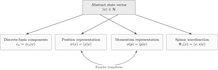
One abstract vector $|\psi\rangle$ has many coordinate descriptions. Position and momentum wavefunctions, discrete components, and spinor-valued wavefunctions are representations of the same state, not competing kinds of state. Transforming every object consistently leaves physical predictions unchanged.

From Discrete Components to a Wavefunction

In an orthonormal discrete basis $\{|e_n\rangle\}$, a state has components

$$c_n=\langle e_n|\psi\rangle$$

and the expansion

$$|\psi\rangle = \sum_n c_n|e_n\rangle.$$

The position representation is the continuous analogue. Formally, position labels a generalized basis $\{|x\rangle\}$ with

$$\langle x|x'\rangle=\delta(x-x')$$

and resolution of the identity

$$I = \int_{-\infty}^{\infty} dx\,|x\rangle\langle x|.$$

Inserting this identity gives

$$\begin{aligned} |\psi\rangle &= \int_{-\infty}^{\infty} dx\,|x\rangle\langle x|\psi\rangle \\ &= \int_{-\infty}^{\infty} dx\,\psi(x)|x\rangle. \end{aligned}$$

Thus $\psi(x)$ plays the same coordinate role as $c_n$. A sum has become an integral, Kronecker orthogonality has become delta normalization, and a list of components has become a function.

The notation is compact but formal. Exact position kets are not ordinary finite-norm vectors, so these identities are interpreted through the spectral theorem or in a rigged Hilbert space. The practical and rigorous viewpoints are developed in Generalized Eigenvectors and Rigged Hilbert Spaces, First Look.

Position Eigenkets Are Generalized Vectors

For the position operator $X$, the symbolic eigenvalue equation is

$$X|x\rangle=x|x\rangle.$$

If $X$ has continuous spectrum, $|x\rangle$ is not normally an element of the physical Hilbert space. Its delta normalization already signals this:

$$\langle x|x\rangle=\delta(0),$$

which is not a finite norm. The ket $|x\rangle$ is instead a generalized spectral vector used under pairings and integrals.

This distinction separates two objects that are easy to conflate:

• $|\psi\rangle$ is a normalizable state vector when $\psi$ is a physical pure state;
• $|x\rangle$ is an idealized generalized eigenket labelling one point of a continuous spectrum.

An exactly localized position eigenket is therefore not an ordinary physical state. Normalizable wave packets can be sharply localized, but they have a nonzero spatial width.

The Representation Map

Let $R_x$ denote the map that sends an abstract vector to its position-space representative:

$$(R_x|\psi\rangle)(x) = \langle x|\psi\rangle.$$

For the elementary particle on the line, this map identifies the abstract Hilbert space with $L^2(\mathbb R,dx)$ up to the usual almost-everywhere equivalence of functions. It preserves inner products:

$$\langle\phi|\psi\rangle = \int_{-\infty}^{\infty} dx\,\phi(x)^*\psi(x).$$

Consequently it preserves norms:

$$\|\psi\|^2 = \langle\psi|\psi\rangle = \int_{-\infty}^{\infty} dx\,|\psi(x)|^2.$$

In mathematical language, a complete position representation is unitary from the abstract Hilbert space onto an appropriate function space. The word “unitary” here means that the change of description loses no information and preserves the Hilbert-space geometry.

The bra coordinate is the complex conjugate:

$$\langle\psi|x\rangle = \langle x|\psi\rangle^* = \psi(x)^*.$$

This relation follows from the adjoint operation, not from a separate probability postulate.

Probability Density Is Measure-Relative

For a normalized state on the line, the position Born rule reads

$$\Pr(x\in\Delta) = \int_\Delta dx\,|\psi(x)|^2$$

for a measurable region $\Delta$. Thus $|\psi(x)|^2$ is a probability density with respect to the measure $dx$.

The phrase “with respect to” matters. A density is not itself a probability, and its numerical value depends on the coordinate and measure used. In one dimension,

$$[|\psi(x)|^2]=L^{-1}, \qquad [\psi(x)]=L^{-1/2},$$

so that $|\psi(x)|^2dx$ is dimensionless. The probability of one exact point is normally zero even when the density there is nonzero:

$$\Pr(X=x_0)=0$$

for an absolutely continuous position distribution.

The full measure-theoretic Born rule, including spectral projectors and mixed states, belongs to Born Rule for Continuous Spectra.

Coordinates, Jacobians, and Measures

The simple expression $|\psi(x)|^2dx$ uses Cartesian position and Lebesgue measure. In general coordinates $q=(q^1,\ldots,q^d)$, the inner product may be

$$\langle\phi|\psi\rangle = \int dq\,J(q)\phi(q)^*\psi(q),$$

where $J(q)$ is the Jacobian density. Then

$$d\Pr(q) = J(q)|\psi(q)|^2dq.$$

For example, in spherical coordinates in three dimensions,

$$d^3r = r^2\sin\theta\,dr\,d\theta\,d\varphi.$$

One may instead absorb the square root of the Jacobian into a redefined coordinate function. If

$$\widetilde\psi(q) = J(q)^{1/2}\psi(q),$$

then the same norm becomes

$$\langle\psi|\psi\rangle = \int dq\,|\widetilde\psi(q)|^2.$$

Both conventions are valid, but formulas for operators and boundary conditions must be transformed consistently. Writing a density without its measure hides information needed to interpret it.

More abstractly, a spectral representation can have the form

$$\mathcal H \simeq \int_X^{\oplus} \mathcal K_x\,d\mu(x),$$

where $d\mu$ is a spectral measure and $\mathcal K_x$ accounts for degeneracy or internal multiplicity. The elementary scalar wavefunction is the special case in which almost every fiber $\mathcal K_x$ is one dimensional.

Wavefunction Versus State Vector

The relation between an abstract vector and a wavefunction can be summarized without identifying them:

• $|\psi\rangle$ does not depend on a chosen basis or coordinate chart;
• $\psi(x)=\langle x|\psi\rangle$ depends on the chosen generalized basis, its phase convention, and its measure convention;
• the norm, transition probabilities, and expectation values do not depend on that choice when all represented objects are transformed together;
• a different wavefunction can therefore describe the same abstract vector in a different representation;
• multiplying one fixed-representation wavefunction by an arbitrary function is generally a change of state, not merely a change of notation.

There are two layers of equivalence. First, $L^2$ functions that differ only on a set of measure zero represent the same Hilbert-space vector. Second, normalized vectors that differ by a constant phase represent the same physical pure-state ray:

$$\psi'(x)=e^{i\alpha}\psi(x), \qquad \alpha\text{ independent of }x.$$

These are different statements. Almost-everywhere equivalence is built into the function space, whereas global-phase equivalence is the passage from a normalized vector to a physical ray.

Point Values and L2 Equivalence

An element of $L^2(\mathbb R)$ is an equivalence class of functions, not a preferred pointwise function. If $\psi$ and $\widetilde\psi$ differ only on a set of measure zero, then

$$\|\psi-\widetilde\psi\|_2=0,$$

so they represent the same vector. Changing a wavefunction at one isolated point does not change any probability obtained by integration.

This fact qualifies the informal phrase “the amplitude at exactly $x$.” The notation $\psi(x)=\langle x|\psi\rangle$ is invaluable, but point evaluation is not a well-defined continuous operation on arbitrary $L^2$ equivalence classes. In applications, differential equations and regularity conditions often select a continuous or differentiable representative on which pointwise expressions make sense.

The distinction becomes important when discussing derivatives, boundary values, singular potentials, and operator domains. Square integrability alone does not guarantee that $d\psi/dx$ exists or that a boundary value is defined.

Other Continuous Representations

Position is only one continuous observable. Given a generalized basis $\{|a,\lambda\rangle\}$, where $a$ is a continuous spectral value and $\lambda$ resolves degeneracy, define

$$\psi_\lambda(a) = \langle a,\lambda|\psi\rangle.$$

The identity resolution takes the schematic form

$$I = \sum_\lambda \int d\mu(a)\, |a,\lambda\rangle\langle a,\lambda|,$$

and reconstruction becomes

$$|\psi\rangle = \sum_\lambda \int d\mu(a)\, \psi_\lambda(a)|a,\lambda\rangle.$$

The word “wavefunction” is often used broadly for any such complex amplitude function. Context should identify the spectral variable, measure, and any degeneracy labels.

Mixed discrete and continuous spectra require both sums and integrals. Bound energy levels, scattering energies, angular-momentum labels, channel indices, and internal quantum numbers may all appear in one representation.

Momentum-Space Wavefunction

The momentum-space representative of the same state is

$$\phi(p)=\langle p|\psi\rangle.$$

With the site’s one-dimensional Fourier convention,

$$\phi(p) = \frac{1}{\sqrt{2\pi\hbar}} \int_{-\infty}^{\infty} dx\,e^{-ipx/\hbar}\psi(x),$$

and

$$\psi(x) = \frac{1}{\sqrt{2\pi\hbar}} \int_{-\infty}^{\infty} dp\,e^{ipx/\hbar}\phi(p).$$

These are not two states. They are two complete coordinate descriptions of one state, related by a unitary transform. In particular,

$$\int dx\,|\psi(x)|^2 = \int dp\,|\phi(p)|^2.$$

The detailed momentum-basis construction, operator actions, and plane-wave caveats are canonical in Momentum-Space Representation. The precise phase and normalization choices are fixed in Fourier Transform Conventions.

Changing Between General Representations

Suppose $|a\rangle$ and $|b\rangle$ label two complete generalized bases. The overlap kernel

$$K(b,a)=\langle b|a\rangle$$

transforms one wavefunction into the other:

$$\begin{aligned} \psi_b(b) &= \langle b|\psi\rangle \\ &= \int d\mu(a)\, \langle b|a\rangle\langle a|\psi\rangle \\ &= \int d\mu(a)\, K(b,a)\psi_a(a). \end{aligned}$$

The Fourier kernel is the position-to-momentum example:

$$\langle p|x\rangle = \frac{1}{\sqrt{2\pi\hbar}} e^{-ipx/\hbar}.$$

A representation change is therefore an integral-kernel analogue of matrix multiplication. It is passive: the abstract state remains fixed while its coordinates change. An active unitary transformation instead changes the state vector and therefore changes its coordinate function unless a symmetry or convention identifies the outcomes.

Operators in a Wavefunction Representation

An abstract operator $A$ becomes a rule acting on representative functions. Its position-space kernel is

$$A(x,x')=\langle x|A|x'\rangle,$$

and formally

$$(A\psi)(x) = \int dx'\,A(x,x')\psi(x').$$

For familiar canonical operators on the line,

$$(X\psi)(x)=x\psi(x)$$

and, on a suitable domain,

$$(P\psi)(x) = -i\hbar\frac{d\psi}{dx}.$$

The expectation value has the same abstract and represented forms:

$$\begin{aligned} \langle A\rangle_\psi &= \langle\psi|A|\psi\rangle \\ &= \int dx\,\psi(x)^*(A\psi)(x). \end{aligned}$$

The differential expression alone is not always the complete operator. Boundary conditions, domains, and the measure in the inner product affect self-adjointness and physical predictions. Those operator-centered issues belong to Operator Representations and Hermitian vs Self-Adjoint Operators.

Time Dependence

In the Schrödinger picture with a fixed position basis,

$$\psi(x,t) = \langle x|\psi(t)\rangle.$$

The time dependence belongs to the state vector, so projecting the abstract Schrödinger equation onto $\langle x|$ produces its position-space form. For a standard one-particle Hamiltonian,

$$i\hbar\frac{\partial\psi}{\partial t} = \left( -\frac{\hbar^2}{2m}\frac{\partial^2}{\partial x^2} +V(x,t) \right)\psi.$$

This equation governs the coordinates of the evolving vector; it does not turn the coordinate function into a basis-independent object. If the basis itself depends on time, differentiating the components produces additional terms from the changing basis. The dynamical postulates and solution methods are treated in Schrödinger Equation and Wave-Mechanics Postulates.

Spatial Phase Carries State Information

The position density does not determine a pure state. Write

$$\psi(x)=R(x)e^{iS(x)}, \qquad R(x)\ge0.$$

Then $|\psi(x)|^2=R(x)^2$ contains no direct information about $S(x)$, yet the phase affects interference and momentum. When boundary terms vanish,

$$\langle P\rangle = \int dx\, \psi(x)^* \left(-i\hbar\frac{d}{dx}\right) \psi(x).$$

For sufficiently regular real $\theta$ and $\psi$, replacing $\psi(x)$ by $e^{i\theta(x)}\psi(x)$ leaves the position density unchanged but shifts the momentum expectation by

$$\Delta\langle P\rangle = \hbar \int dx\,|\psi(x)|^2\theta'(x).$$

Only a constant $\theta$ is an ordinary global-phase change. A local phase may participate in a gauge transformation when the electromagnetic potentials are transformed at the same time; multiplying the wavefunction alone by an arbitrary local phase is not generally a redundancy.

Example: A Gaussian Wave Packet

Consider

$$\psi(x) = \frac{1}{(2\pi\sigma^2)^{1/4}} \exp\left[ -\frac{(x-x_0)^2}{4\sigma^2} +ik_0x \right].$$

Its position density is

$$|\psi(x)|^2 = \frac{1}{\sqrt{2\pi\sigma^2}} \exp\left[ -\frac{(x-x_0)^2}{2\sigma^2} \right].$$

The parameter $x_0$ is the mean position and $\sigma^2$ is the position variance. The factor $e^{ik_0x}$ does not change this position density, but it shifts the mean momentum to $\hbar k_0$. This is a simple demonstration that a wavefunction carries more information than its modulus squared in one chosen representation.

The packet is a normalizable Hilbert-space state. An ideal plane wave $e^{ik_0x}$ is not: its modulus is constant over the whole line, so its norm diverges. Plane waves instead serve as generalized momentum eigenfunctions inside wave-packet expansions.

Configuration Space Is Not Always Physical Space

For one spinless particle in three dimensions,

$$\psi(\mathbf r) = \langle\mathbf r|\psi\rangle$$

is a scalar function on physical space. For $N$ distinguishable particles, the position representation is instead

$$\Psi(\mathbf r_1,\ldots,\mathbf r_N) = \langle \mathbf r_1,\ldots,\mathbf r_N |\Psi\rangle,$$

a function on a $3N$-dimensional configuration space. Its normalization is

$$\int \prod_{j=1}^{N}d^3r_j\, |\Psi(\mathbf r_1,\ldots,\mathbf r_N)|^2 =1.$$

The many-particle wavefunction should therefore not be pictured naively as a single classical field living in ordinary three-dimensional space. For identical particles it also obeys symmetry or antisymmetry conditions under particle exchange. Those structures belong to Identical Particles.

Internal Degrees of Freedom

Position may not be a complete set of labels. A spin-$1/2$ particle has a two-component position-space wavefunction

$$\Psi(x) = \begin{pmatrix} \psi_\uparrow(x)\\ \psi_\downarrow(x) \end{pmatrix},$$

where

$$\psi_s(x)=\langle x,s|\Psi\rangle, \qquad s\in\{\uparrow,\downarrow\}.$$

The total position density when spin is not resolved is

$$\rho(x) = |\psi_\uparrow(x)|^2 + |\psi_\downarrow(x)|^2.$$

If the two components are proportional to one common spatial function, the state factors into spatial and spin parts. In general they need not be proportional, and spin can be entangled with position. A wavefunction can thus be scalar-valued, vector-valued, or carry still richer internal indices.

Mixed States Require More Than One Wavefunction

A single normalized wavefunction represents a pure state vector. A general mixed state is represented by a density operator $\rho$, not by one wavefunction. In position representation its kernel is

$$\rho(x,x') = \langle x|\rho|x'\rangle.$$

For a pure state,

$$\rho_\psi(x,x') = \psi(x)\psi(x')^*.$$

For a mixture written as

$$\rho = \sum_k p_k|\psi_k\rangle\langle\psi_k|,$$

the kernel is

$$\rho(x,x') = \sum_k p_k \psi_k(x)\psi_k(x')^*.$$

Its diagonal gives the position probability density,

$$\rho(x,x)=\langle x|\rho|x\rangle,$$

while off-diagonal entries encode spatial coherence in that representation. Different ensembles can yield the same density operator, so the individual $\psi_k$ in an ensemble decomposition are not uniquely determined by the mixed state. See Density Operators for the canonical mixed-state treatment.

What Remains Invariant

Changing representation can alter the visible form of nearly every formula:

• a column becomes a function;
• a matrix becomes a differential operator or integral kernel;
• a sum becomes an integral;
• a Kronecker delta becomes a Dirac delta;
• a flat measure may acquire a Jacobian;
• a scalar wavefunction may become a multi-component function.

The following quantities remain unchanged under a unitary representation change:

$$\begin{gathered} \langle\phi|\psi\rangle, \qquad \|\psi\|, \qquad \langle\psi|A|\psi\rangle,\\ \Pr(\text{measurement event}), \qquad \operatorname{spec}(A). \end{gathered}$$

The represented function by itself is not invariant. Trustworthy calculations transform the state, operators, measure, and boundary data as one consistent package.

Practical Interpretation Checklist

When a wavefunction appears, identify:

1. State type. Is it a normalizable pure state, one member of an ensemble, or a generalized eigenfunction?
2. Representation. What variable or observable labels the components?
3. Measure. Is the norm integrated with $dx$, $d^3r$, a Jacobian-weighted measure, or a spectral measure?
4. Internal labels. Are spin, band, channel, or degeneracy indices suppressed?
5. Domain. What region, regularity conditions, and boundary conditions are assumed?
6. Convention. What phases and normalization are used for the generalized basis?
7. Physical question. Which measurement does the modulus squared describe, and which operator represents other observables?

This checklist prevents notation such as $\psi(x)$ from carrying more meaning than has actually been specified.

Common Mistakes

• Treating the position-space wavefunction as the abstract state itself.
• Assuming every quantum state is described by one scalar function on physical three-dimensional space.
• Treating $|\psi(x)|^2$ as a probability rather than a density relative to a specified measure.
• Forgetting that continuous-spectrum kets are generalized vectors, not normalizable states.
• Assuming two $L^2$ representatives that differ at one point are different Hilbert-space vectors.
• Believing that the position density determines the phase or the full pure state.
• Calling an arbitrary position-dependent phase a global phase.
• Using a differential expression without specifying its domain and boundary conditions.
• Forgetting spin, channel, degeneracy, or particle labels hidden inside a multi-component wavefunction.
• Trying to represent a general mixed state by a single wavefunction.

Scope and Canonical Neighbors

This page owns the conceptual statement that a wavefunction is a representation of an abstract state. It does not duplicate the full calculation machinery found elsewhere:

• Normalization develops ordinary, delta, and box normalization;
• Born Rule for Continuous Spectra develops interval probabilities and spectral measures;
• Momentum-Space Representation develops momentum wavefunctions and Fourier conventions;
• Operator Representations develops matrices, kernels, and differential forms;
• Coordinate Representation applies the framework in wave-mechanics calculations;
• L2 Spaces develops the function-space mathematics behind normalizable wavefunctions.

References

• P. A. M. Dirac, The Principles of Quantum Mechanics, 4th ed., Oxford University Press, 1958, Chapters II and III.
• J. J. Sakurai and J. Napolitano, Modern Quantum Mechanics, 3rd ed., Cambridge University Press, 2021, Chapters 1 and 2.
• R. Shankar, Principles of Quantum Mechanics, 2nd ed., Springer, 1994, Chapters 1, 4, and 5.
• L. E. Ballentine, Quantum Mechanics: A Modern Development, 2nd ed., World Scientific, 2014, Chapters 2 and 3.
• B. C. Hall, Quantum Theory for Mathematicians, Springer, 2013, Chapters 3, 7, and 10.
• M. Reed and B. Simon, Methods of Modern Mathematical Physics, Volume I: Functional Analysis, revised and enlarged ed., Academic Press, 1980, Sections II.2 and VII.3.

Exercises

1. Reconstruction and inner products

Assume the formal position completeness relation. Starting from $\psi(x)=\langle x|\psi\rangle$, reconstruct $|\psi\rangle$ and derive the position-space formula for $\langle\phi|\psi\rangle$.

Solution

Insert the identity:

$$\begin{aligned} |\psi\rangle &=I|\psi\rangle \\ &= \int dx\,|x\rangle\langle x|\psi\rangle \\ &= \int dx\,\psi(x)|x\rangle. \end{aligned}$$

Then

$$\begin{aligned} \langle\phi|\psi\rangle &= \int dx\, \langle\phi|x\rangle \langle x|\psi\rangle \\ &= \int dx\,\phi(x)^*\psi(x). \end{aligned}$$

The second equality uses $\langle\phi|x\rangle=\langle x|\phi\rangle^*=\phi(x)^*$.

2. Units of a many-particle wavefunction

Find the physical dimensions of a normalized position-space wavefunction for $N$ particles in $d$ spatial dimensions. Assume Cartesian coordinates.

Solution

Normalization requires

$$1 = \int \prod_{j=1}^{N}d^dr_j\, |\Psi(\mathbf r_1,\ldots,\mathbf r_N)|^2.$$

The product measure has dimensions $L^{dN}$. Therefore

$$[|\Psi|^2]=L^{-dN}$$

and

$$[\Psi]=L^{-dN/2}.$$

This dimensional statement refers to the chosen Cartesian position representation, not to the abstract state vector.

3. Absorbing a radial Jacobian

Let $\psi(\mathbf r)=R(r)Y_{\ell m}(\theta,\varphi)$, with spherical harmonics normalized on the unit sphere. Show that the three-dimensional norm reduces to $\int_0^\infty dr\,r^2|R(r)|^2$, and define a reduced radial function whose norm uses the flat measure $dr$.

Solution

Using $d^3r=r^2dr\,d\Omega$ and $\int d\Omega\,|Y_{\ell m}|^2=1$ gives

$$\begin{aligned} \|\psi\|^2 &= \int_0^\infty dr\,r^2|R(r)|^2 \int d\Omega\,|Y_{\ell m}|^2 \\ &= \int_0^\infty dr\,r^2|R(r)|^2. \end{aligned}$$

Define

$$u(r)=rR(r).$$

Then

$$\|\psi\|^2 = \int_0^\infty dr\,|u(r)|^2.$$

The Jacobian has moved from the measure into the represented function. The operator acting on $u(r)$ must be transformed consistently as well.

4. Global phase versus spatial phase

Let $\theta$ be real and absolutely continuous, and set $\psi_\theta(x)=e^{i\theta(x)}\psi(x)$. Assume both wavefunctions lie in the momentum operator’s domain. Show that the position density is unchanged and compute the change in $\langle P\rangle$.

Solution

The position density is

$$|\psi_\theta(x)|^2 = |e^{i\theta(x)}|^2|\psi(x)|^2 = |\psi(x)|^2.$$

For momentum,

$$\begin{aligned} -i\hbar\frac{d}{dx} \left(e^{i\theta}\psi\right) &= e^{i\theta} \left( \hbar\theta'\psi -i\hbar\psi' \right). \end{aligned}$$

Therefore

$$\langle P\rangle_{\psi_\theta} = \langle P\rangle_\psi + \hbar\int dx\,|\psi(x)|^2\theta'(x).$$

Because $\theta$ is absolutely continuous, $\theta'(x)=0$ almost everywhere on a connected interval implies that $\theta$ is constant there. In that case the two vectors differ only by global phase.

5. A spinor-valued wavefunction

Suppose

$$\Psi(x) = \begin{pmatrix} f(x)\\ g(x) \end{pmatrix}$$

is normalized. Find the probability of detecting the particle in a region $\Delta$ without resolving spin, and the probability of obtaining spin up along $z$ regardless of position.

Solution

Not resolving spin means summing the mutually exclusive component probabilities:

$$\Pr(x\in\Delta) = \int_\Delta dx\, \left(|f(x)|^2+|g(x)|^2\right).$$

Resolving spin up but not position means integrating the up component over all space:

$$\Pr(\uparrow_z) = \int_{-\infty}^{\infty}dx\,|f(x)|^2.$$

Normalization is

$$\int dx\, \left(|f(x)|^2+|g(x)|^2\right)=1.$$

6. Pure-state density kernel

For a normalized wavefunction $\psi(x)$, verify that $\rho_\psi(x,x')=\psi(x)\psi(x')^*$ has unit trace and is idempotent as an integral kernel.

Solution

The trace is

$$\operatorname{Tr}\rho_\psi = \int dx\,\rho_\psi(x,x) = \int dx\,|\psi(x)|^2 =1.$$

Kernel composition gives

$$\begin{aligned} (\rho_\psi^2)(x,x') &= \int dy\, \rho_\psi(x,y)\rho_\psi(y,x') \\ &= \psi(x)\psi(x')^* \int dy\,|\psi(y)|^2 \\ &= \rho_\psi(x,x'). \end{aligned}$$

Thus the kernel represents the rank-one projector $|\psi\rangle\langle\psi|$.

7. Same vector, different L2 representatives

Let $\widetilde\psi(x)=\psi(x)$ for every $x\ne0$, but set $\widetilde\psi(0)=10^{100}$. Do these functions represent different vectors in $L^2(\mathbb R)$? Do they predict different interval probabilities?

Solution

They differ only on the one-point set $\{0\}$, which has Lebesgue measure zero. Hence

$$\int dx\, |\widetilde\psi(x)-\psi(x)|^2 =0.$$

They are the same element of $L^2(\mathbb R)$ and give the same probability for every measurable interval. This example also shows why arbitrary point values cannot be intrinsic data of an $L^2$ state.

8. Representation-invariant expectation value

Let $R$ be a unitary representation map, with $\psi_R=R|\psi\rangle$ and $A_R=RAR^{-1}$. Prove that evaluating the expectation value in the representation gives the abstract result.

Solution

Because $R$ is unitary, $R^{-1}=R^\dagger$. Therefore

$$\begin{aligned} \langle\psi_R,A_R\psi_R\rangle_R &= \langle R\psi, RAR^{-1}R\psi\rangle_R \\ &= \langle R\psi,RA\psi\rangle_R \\ &= \langle\psi,A\psi\rangle_{\mathcal H}. \end{aligned}$$

The represented function and operator both change, while the scalar prediction does not.