Born Rule for Continuous Spectra

For an observable with continuously varying outcomes, the Born rule assigns probabilities to measurable sets of outcomes. A probability density is a useful derivative of that probability law when such a derivative exists; it is not the probability of an exact value.

This distinction is easy to blur in notation. The familiar statement $p(x)=|\psi(x)|^2$ is correct for position in the standard representation, but the logically prior statement is

$$\Pr(A\in\Delta) = \operatorname{Tr}\!\left[\rho P^A(\Delta)\right],$$

where $P^A(\Delta)$ is the spectral projector associated with a measurable set $\Delta\subseteq\mathbb R$. This page develops densities, interval probabilities, coordinate changes, mixed spectra, and finite resolution from that measure-first formulation. The general probability postulate lives at Born Rule; the companion page Born Rule for Discrete Spectra handles countable outcomes.

Required background. The Born Rule supplies probabilities for measurement events.

Helpful background. Wavefunctions as Representations supplies continuous-basis amplitudes; Spectra distinguishes discrete, continuous, and mixed cases. Familiarity with integrating probability densities and transforming them with Jacobians is assumed.

Why probabilities belong to sets

A measuring device reports an event in a set: a pixel, an energy channel, a time window, or a numerical bin. The probability of that event is the measure of the set. A density value is not itself a probability and is defined only almost everywhere, so it depends on the chosen representative and reference measure. Sets are therefore both the mathematically natural events and the experimentally natural ones.

Let $A$ be self-adjoint, let $P^A$ be its projection-valued measure, and let $\rho$ be a density operator. Define

$$\mu_\rho^A(\Delta) \equiv \operatorname{Tr}\!\left[\rho P^A(\Delta)\right]$$

for each Borel set $\Delta\subseteq\mathbb R$. The map $\mu_\rho^A$ is a probability measure:

$$\begin{aligned} \mu_\rho^A(\Delta)&\ge 0,\\ \mu_\rho^A(\mathbb R)&=1,\\ \mu_\rho^A\!\left(\bigcup_{n=1}^{\infty}\Delta_n\right) &= \sum_{n=1}^{\infty}\mu_\rho^A(\Delta_n) \end{aligned}$$

whenever the sets $\Delta_n$ are pairwise disjoint. For a pure state, $\rho=|\psi\rangle\langle\psi|$, this becomes

$$\mu_\psi^A(\Delta) = \langle\psi|P^A(\Delta)|\psi\rangle.$$

The observable supplies the spectral projectors; the state supplies their probabilities. Consequently, the relevant probability law is always state-dependent even though the spectrum of $A$ is not.

From a probability measure to a density

Suppose the spectral probability measure is absolutely continuous with respect to Lebesgue measure $d\lambda$. Then there is a nonnegative function $p_A(\lambda)$, defined up to changes on sets of Lebesgue measure zero, such that

$$\mu_\rho^A(\Delta) = \int_\Delta p_A(\lambda)\,d\lambda.$$

In measure-theoretic language, the density is the Radon–Nikodym derivative

$$p_A(\lambda) = \frac{d\mu_\rho^A}{d\lambda}(\lambda).$$

It obeys

$$p_A(\lambda)\ge 0, \qquad \int_{-\infty}^{\infty}p_A(\lambda)\,d\lambda=1.$$

If $\lambda$ carries physical units $[\lambda]$, then $p_A$ has units $[\lambda]^{-1}$. Only the product $p_A(\lambda)d\lambda$ is a dimensionless probability.

Not every spectral measure admits a density with respect to $d\lambda$. Discrete components give atoms, and singular-continuous measures can occur in more specialized spectral problems. The measure $\mu_\rho^A$ is always the safe starting point; a density is an additional representation of its absolutely continuous part.

Probability is area, not height

When a density exists, an interval probability is the area under the density:

$$\Pr(a\le A\le b) = \int_a^b p_A(\lambda)\,d\lambda.$$

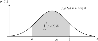
For an absolutely continuous probability law, the shaded area is $\Pr(A\in[a,b])$. The height $p_A(\lambda_0)$ is a density, not the probability of the exact value $\lambda_0$; an atomic component would have to be represented separately.

A narrow bin of width $\Delta\lambda$ centered at $\lambda_0$ has probability

$$\begin{aligned} &\Pr\!\left( \lambda_0-\frac{\Delta\lambda}{2} \le A \le \lambda_0+\frac{\Delta\lambda}{2} \right)\\ &\qquad= \int_{\lambda_0-\Delta\lambda/2}^{\lambda_0+\Delta\lambda/2} p_A(\lambda)\,d\lambda. \end{aligned}$$

If $p_A$ is continuous near $\lambda_0$ and the bin is sufficiently narrow,

$$\Pr(A\text{ in the bin}) = p_A(\lambda_0)\Delta\lambda +o(\Delta\lambda).$$

This local approximation explains why histograms estimate density by dividing bin frequencies by bin width.

Exact values, null sets, and atoms

For an absolutely continuous probability law,

$$\Pr(A=\lambda_0) = \mu_\rho^A(\{\lambda_0\}) =0.$$

The conclusion follows because a singleton has zero Lebesgue measure. It does not mean that the measurement cannot return a numerical value. It means that no preselected exact value has positive probability under the idealized continuous law.

The qualifier “absolutely continuous” matters. For any self-adjoint $A$,

$$P^A(\{\lambda_0\})$$

is the projector onto the eigenspace at $\lambda_0$. If the state has a nonzero component in that eigenspace, then

$$\Pr(A=\lambda_0) = \operatorname{Tr}\!\left[ \rho P^A(\{\lambda_0\}) \right] >0.$$

Such a point mass is called an atom. An observable can have bound-state eigenvalues and a scattering continuum at the same time, so the slogan “exact values have probability zero” must never be applied indiscriminately to a mixed spectrum.

Endpoint conventions

For a purely absolutely continuous law, the intervals $[a,b]$, $(a,b)$, $[a,b)$, and $(a,b]$ have the same probability because their differences are singletons. Thus

$$\mu_\rho^A([a,b]) = \mu_\rho^A((a,b))$$

in that case.

If an endpoint is an atom, brackets matter. For example, if $\mu_\rho^A(\{a\})=w$, then

$$\mu_\rho^A([a,b]) - \mu_\rho^A((a,b]) =w.$$

This is one reason spectral events should be written as explicit sets rather than inferred from an integral alone.

Position as the standard example

For a normalized one-dimensional wavefunction $\psi(x)=\langle x|\psi\rangle$,

$$\int_{-\infty}^{\infty}|\psi(x)|^2\,dx=1.$$

The position density with respect to $dx$ is

$$p_X(x)=|\psi(x)|^2,$$

and therefore

$$\Pr(X\in\Delta) = \int_\Delta |\psi(x)|^2\,dx.$$

In the position representation, the spectral projector acts by multiplying a wavefunction by the indicator function of the set:

$$\bigl(P^X(\Delta)\psi\bigr)(x) = \mathbf 1_\Delta(x)\psi(x).$$

It follows directly that

$$\begin{aligned} \langle\psi|P^X(\Delta)|\psi\rangle &= \int_{-\infty}^{\infty} \psi^*(x)\mathbf 1_\Delta(x)\psi(x)\,dx\\ &= \int_\Delta |\psi(x)|^2\,dx. \end{aligned}$$

The density $|\psi(x)|^2$ has units of inverse length in one dimension. Its value at one isolated point can be changed without changing the physical state as an element of $L^2(\mathbb R)$ or changing any interval probability.

Generalized eigenvectors and delta normalization

The notation

$$P^X(\Delta) = \int_\Delta |x\rangle\langle x|\,dx$$

is a useful generalized-basis expression. It is not a sum over normalizable Hilbert-space vectors. The position kets satisfy the distributional relations

$$\begin{aligned} \langle x|x'\rangle &= \delta(x-x'),\\ \int_{-\infty}^{\infty}|x\rangle\langle x|\,dx &=I, \end{aligned}$$

interpreted in the appropriate weak or rigged-Hilbert-space sense. The delta function and generalized eigenvectors have their own canonical treatments.

More generally, suppose a continuous spectral sector is labeled by $\lambda$ and a discrete degeneracy index $\alpha$. With the convention

$$\langle\lambda,\alpha|\lambda',\alpha'\rangle = \delta_{\alpha\alpha'}\delta(\lambda-\lambda'),$$

write

$$c_\alpha(\lambda) = \langle\lambda,\alpha|\psi\rangle.$$

Then the density with respect to $d\lambda$ is

$$p_A(\lambda) = \sum_\alpha |c_\alpha(\lambda)|^2,$$

with an integral replacing the sum if the degeneracy label is itself continuous. The amplitudes inherit units from the delta-normalization convention; $|c_\alpha(\lambda)|^2d\lambda$ is dimensionless.

Momentum probability density

In the momentum representation,

$$\phi(p) = \langle p|\psi\rangle, \qquad \int_{-\infty}^{\infty}|\phi(p)|^2\,dp=1.$$

Thus

$$\begin{aligned} p_P(p)&=|\phi(p)|^2,\\ \Pr(P\in\Delta) &= \int_\Delta |\phi(p)|^2\,dp. \end{aligned}$$

The ket $|p\rangle$ is delta-normalized, whereas a physical wave packet $|\psi\rangle$ is normalizable. The Fourier transform relating $\phi(p)$ and $\psi(x)$ depends on convention, but a consistent convention always preserves normalization. See Momentum-Space Representation for that transformation and its factors of $2\pi$ and $\hbar$.

Densities change under relabeling

A density is always a density with respect to a specified measure and variable. Let $Y=g(X)$, with $g$ differentiable and monotone on the relevant domain. Conservation of probability gives

$$p_X(x)\,dx = p_Y(y)\,dy,$$

so

$$p_Y(y) = p_X\!\left(g^{-1}(y)\right) \left| \frac{d g^{-1}}{dy} \right|.$$

If several inverse branches $x_i(y)$ contribute, their probabilities add:

$$p_Y(y) = \sum_{i:g(x_i)=y} p_X(x_i(y)) \left| \frac{dx_i}{dy} \right|.$$

This formula is the continuous analogue of summing probabilities over distinct fine-grained outcomes that produce the same coarse-grained result.

For example, $p=\hbar k$ implies

$$p_K(k) = \hbar\,p_P(\hbar k),$$

not merely $p_P(\hbar k)$. The factor of $\hbar$ supplies the Jacobian and the correct units.

Worked example: a Gaussian interval

Consider the normalized density

$$p_X(x) = \frac{1}{\sqrt{2\pi}\sigma} \exp\!\left[-\frac{(x-x_c)^2}{2\sigma^2}\right].$$

For an interval centered at $x_c$ with half-width $L$,

$$\begin{aligned} \Pr(|X-x_c|\le L) &= \int_{x_c-L}^{x_c+L}p_X(x)\,dx\\ &= \operatorname{erf}\!\left( \frac{L}{\sqrt{2}\sigma} \right). \end{aligned}$$

The density at the center is $p_X(x_c)=1/(\sqrt{2\pi}\sigma)$, which can exceed one when $\sigma$ is small. There is no contradiction: a density is not constrained to be at most one. Only integrated probabilities must lie in $[0,1]$.

Free-particle energy and degeneracy

For a one-dimensional free particle,

$$E = \frac{p^2}{2m}, \qquad E\ge 0.$$

Every $E>0$ receives contributions from two momentum values, $p=\pm\sqrt{2mE}$. Applying the many-branch change-of-variable rule gives

$$\begin{aligned} p_E(E) &= \frac{m}{p_\star(E)} \biggl[ p_P\!\left(p_\star(E)\right) \\ &\qquad +p_P\!\left(-p_\star(E)\right) \biggr],\\ p_\star(E)&=\sqrt{2mE}, \qquad E>0. \end{aligned}$$

The factor $m/\sqrt{2mE}$ is the Jacobian $|dp/dE|$. The two terms are the right-moving and left-moving degeneracy branches. Although the density may have an integrable $E^{-1/2}$ behavior near zero, normalization is preserved:

$$\int_0^\infty p_E(E)\,dE = \int_{-\infty}^{\infty}p_P(p)\,dp =1.$$

In higher dimensions or in scattering with internal channels, direction, angular momentum, polarization, or spin can provide additional degeneracy labels. One must sum or integrate over every unobserved label.

Three-dimensional position measurements

For a wavefunction $\psi(\mathbf r)$ normalized with respect to Euclidean volume,

$$\int_{\mathbb R^3}|\psi(\mathbf r)|^2\,d^3r=1,$$

the probability of a spatial region $R$ is

$$\Pr(\mathbf X\in R) = \int_R |\psi(\mathbf r)|^2\,d^3r.$$

Here $|\psi(\mathbf r)|^2$ is a density with respect to the geometric volume measure $d^3r$, not with respect to an arbitrary triple of coordinate differentials.

In spherical coordinates,

$$d^3r = r^2\sin\theta\,dr\,d\theta\,d\phi,$$

so

$$\begin{aligned} \Pr(\mathbf X\in R) &= \int_R |\psi(r,\theta,\phi)|^2\\ &\qquad{} \times r^2\sin\theta\,dr\,d\theta\,d\phi. \end{aligned}$$

The factor $r^2\sin\theta$ is a coordinate Jacobian. Omitting it changes the probability measure.

Marginal and radial densities

If an experiment records only the radius, angular outcomes must be integrated out. The radial density with respect to $dr$ is

$$\begin{aligned} p_R(r) &= r^2\int_{S^2}|\psi(r,\Omega)|^2\,d\Omega,\\ d\Omega &= \sin\theta\,d\theta\,d\phi, \qquad r\ge0. \end{aligned}$$

It satisfies

$$\begin{aligned} \Pr(r\in[a,b]) &= \int_a^b p_R(r)\,dr,\\ \int_0^\infty p_R(r)\,dr &=1. \end{aligned}$$

For a separated central-potential state

$$\psi(r,\theta,\phi) = R_{n\ell}(r)Y_{\ell m}(\theta,\phi)$$

with normalized spherical harmonic, the radial density is

$$p_R(r) = r^2|R_{n\ell}(r)|^2.$$

Thus $|R_{n\ell}(r)|^2$ alone is not the probability density for radius. If one instead defines the reduced radial function $u_{n\ell}(r)=rR_{n\ell}(r)$, then $|u_{n\ell}(r)|^2$ is the radial density with respect to $dr$.

Density operators in a continuous basis

For a mixed state, let

$$\rho(x,x') = \langle x|\rho|x'\rangle$$

be the position-space kernel. The position probability is

$$\begin{aligned} \Pr(X\in\Delta) &= \operatorname{Tr}\!\left[ \rho P^X(\Delta) \right]\\ &= \int_\Delta \rho(x,x)\,dx. \end{aligned}$$

Therefore

$$p_X(x)=\rho(x,x).$$

Positivity of $\rho$ ensures $\rho(x,x)\ge0$ in the usual kernel sense, and unit trace gives

$$\int_{-\infty}^{\infty}\rho(x,x)\,dx=1.$$

The diagonal depends on the chosen basis. Position probabilities use the position-basis diagonal; momentum probabilities use $\langle p|\rho|p\rangle$. Off-diagonal elements encode coherence and affect probabilities in other measurement bases even though they do not appear directly in a position measurement.

Mixed discrete and continuous spectra

An observable need not be wholly discrete or wholly continuous. For a state whose spectral measure has discrete weights $w_n$ and an absolutely continuous density $p_{\mathrm{ac}}(\lambda)$, probabilities take the form

$$\mu_\rho^A(\Delta) = \sum_{\lambda_n\in\Delta}w_n + \int_\Delta p_{\mathrm{ac}}(\lambda)\,d\lambda,$$

with

$$\begin{gathered} w_n\ge0, \qquad p_{\mathrm{ac}}(\lambda)\ge0,\\ \sum_n w_n+ \int_{\mathbb R}p_{\mathrm{ac}}(\lambda)\,d\lambda =1. \end{gathered}$$

A Hamiltonian with bound states and scattering states is the standard example. The probability of an exact bound-state energy may be nonzero, while the probability of any preselected scattering energy is zero for an absolutely continuous scattering component.

The page Discrete and Continuous Spectra classifies the operator-level spectral possibilities. The formula above is the corresponding state-level probability decomposition.

Cumulative distributions

The cumulative distribution function is defined directly from the spectral measure:

$$F_A(a) = \Pr(A\le a) = \mu_\rho^A(({-\infty},a]).$$

It is nondecreasing and right-continuous, with limits

$$\lim_{a\to-\infty}F_A(a)=0, \qquad \lim_{a\to\infty}F_A(a)=1.$$

Where an ordinary density exists and $F_A$ is differentiable,

$$p_A(a)=\frac{dF_A}{da}.$$

An atom of weight $w$ appears as a jump of size $w$ in $F_A$. This single object therefore represents discrete, continuous, and mixed probability laws without changing notation.

Expectation values from a density

If the relevant integrals converge, a density determines moments in the usual way:

$$\langle A\rangle_\rho = \int_{-\infty}^{\infty} \lambda p_A(\lambda)\,d\lambda,$$

and

$$(\Delta A)^2 = \int_{-\infty}^{\infty} (\lambda-\langle A\rangle_\rho)^2 p_A(\lambda)\,d\lambda.$$

For a mixed spectrum, add the atomic contributions:

$$\langle A\rangle_\rho = \sum_n \lambda_n w_n + \int_{-\infty}^{\infty} \lambda p_{\mathrm{ac}}(\lambda)\,d\lambda.$$

Normalization alone does not guarantee that the mean or variance is finite. Heavy-tailed spectral distributions can make these moments diverge even though the Born probabilities themselves are well defined. The canonical discussion of moments is at Expectation Values.

Finite detector bins

An ideal binning measurement partitions the outcome axis into disjoint sets $\Delta_j$. Its probabilities are

$$q_j = \mu_\rho^A(\Delta_j) = \int_{\Delta_j}p_A(\lambda)\,d\lambda$$

for an absolutely continuous law. If the bins cover the axis up to a null set,

$$\sum_j q_j=1.$$

This is a genuine discrete distribution produced by coarse-graining a continuous outcome. Refining the bins changes the numbers $q_j$ but not the underlying measure.

A histogram based on $N$ repetitions estimates $q_j$ by $n_j/N$. To estimate a density over a bin of width $h_j$, one plots approximately

$$\widehat p_j = \frac{n_j}{Nh_j}.$$

Without the division by width, the histogram estimates bin probability rather than probability density.

Finite resolution and response functions

Real instruments can blur as well as bin. Let $R(y|\lambda)$ be a conditional response density for recording $y$ when the ideal value is $\lambda$, with

$$R(y|\lambda)\ge0, \qquad \int_{-\infty}^{\infty}R(y|\lambda)\,dy=1.$$

If the ideal law has density $p_A(\lambda)$, the recorded density is

$$q(y) = \int_{-\infty}^{\infty} R(y|\lambda)p_A(\lambda)\,d\lambda.$$

This classical postprocessing preserves normalization:

$$\int_{-\infty}^{\infty}q(y)\,dy=1.$$

More general detectors are described by POVMs and need not be postprocessings of a sharp observable. Their canonical introduction is POVMs: First Encounter. A singleton is a meaningful measurable event and has probability zero for an absolutely continuous law. Finite resolution implements a different event—or, more generally, a smeared POVM effect—rather than turning a density value into an exact-outcome probability.

Discrete and continuous formulas share one structure

For a discrete eigenvalue $a_n$,

$$\Pr(A=a_n) = \operatorname{Tr}(\rho P_n).$$

For a measurable continuous-outcome set $\Delta$,

$$\Pr(A\in\Delta) = \operatorname{Tr}\!\left[ \rho P^A(\Delta) \right].$$

Both statements ask for the expectation value of an event projector. Sums and integrals appear only after choosing a spectral representation:

$$\sum_{a_n\in\Delta} \langle\psi|P_n|\psi\rangle \quad\longleftrightarrow\quad \int_\Delta p_A(\lambda)\,d\lambda.$$

The projector-valued measure, not a symbolic replacement of a sum by an integral, is what unifies the cases.

What a density does and does not mean

A probability density is operationally useful: it predicts relative frequencies in small bins, determines interval probabilities, and allows moments to be calculated when they converge. It should not be reified as a probability attached to a mathematical point.

Several facts follow:

• A density may exceed one and still define a valid probability law.
• The value of a density at one point is physically irrelevant for an absolutely continuous law.
• Densities depend on the coordinate and reference measure used to label outcomes.
• A peak identifies high probability per unit outcome, not necessarily a large probability in a wide comparison region.
• Delta functions represent atomic measure components in density-like notation; they are not ordinary functions of infinite probability.
• The spectrum of the operator and the probability type induced by a particular state are related but should not be conflated.

Common mistakes

Calling the density a probability

Writing $\Pr(X=x)=|\psi(x)|^2$ is dimensionally and conceptually wrong for an ordinary continuous position law. The correct statements are

$$p_X(x)=|\psi(x)|^2$$

and

$$\Pr(X\in\Delta) = \int_\Delta |\psi(x)|^2\,dx.$$

Applying the zero-point rule to atoms

An exact value has zero probability only for a nonatomic component. A bound state, or any point-spectrum component occupied by the state, can carry nonzero probability at one eigenvalue.

Forgetting the Jacobian

Substituting a new variable inside the functional form without transforming the measure generally destroys normalization. Use conservation of probability and include every inverse branch.

Dropping degeneracy labels

An energy density may require a sum over directions, signs of momentum, partial-wave channels, or spin. A density for one channel is not automatically the density for the measured energy alone.

Dropping coordinate-volume factors

In spherical coordinates the density with respect to $dr\,d\theta\,d\phi$ includes $r^2\sin\theta$. The radial density includes the angular marginal and is not generally $|\psi(r)|^2$.

Treating generalized kets as physical states

The kets $|x\rangle$ and $|p\rangle$ are distributionally normalized tools. Physical preparation states are normalizable wave packets or density operators.

Confusing detector resolution with state spread

The ideal density describes the state-dependent outcome law. A detector response function describes additional measurement noise or coarse-graining. The two should be modeled separately before they are convolved.

Summary

For any self-adjoint observable, the Born rule first defines a probability measure

$$\mu_\rho^A(\Delta) = \operatorname{Tr}\!\left[ \rho P^A(\Delta) \right].$$

When its relevant component is absolutely continuous, one may write

$$\mu_\rho^A(\Delta) = \int_\Delta p_A(\lambda)\,d\lambda.$$

The density depends on the chosen outcome variable, transforms with a Jacobian, and has inverse outcome units. Exact values have zero probability for the absolutely continuous component, while atoms can carry nonzero exact-value probability. Generalized eigenvectors provide a compact representation, and finite detector bins recover ordinary discrete probabilities by integrating over specified regions.

References

• P. Busch, P. J. Lahti, J.-P. Pellonpää, and K. Ylinen, Quantum Measurement, Springer, 2016, Chapters 3–5.
• P. A. M. Dirac, The Principles of Quantum Mechanics, 4th ed., Oxford University Press, 1958, Chapters II–III.
• B. C. Hall, Quantum Theory for Mathematicians, Springer, 2013, Chapters 7–10.
• A. Messiah, Quantum Mechanics, Vol. I, North-Holland, 1961, Chapters IV–V.
• M. Reed and B. Simon, Methods of Modern Mathematical Physics, Vol. I: Functional Analysis, revised and enlarged ed., Academic Press, 1980, Sections VII.1–VII.3.
• R. Shankar, Principles of Quantum Mechanics, 2nd ed., Springer, 1994, Chapters 1 and 4.
• J. von Neumann, Mathematical Foundations of Quantum Mechanics, Princeton University Press, 1955, Chapters II–III.

Exercises

1. Uniform wavefunction on an interval

Let

$$\psi(x) = \begin{cases} 1/\sqrt L, & 0\le x\le L,\\ 0, & \text{otherwise}. \end{cases}$$

Find the probability that $X\in[L/4,3L/4]$. State the units of $|\psi(x)|^2$.

Solution

The density is $p_X(x)=1/L$ on $[0,L]$. Therefore

$$\begin{aligned} \Pr\!\left(\frac L4\le X\le\frac{3L}{4}\right) &= \int_{L/4}^{3L/4}\frac{dx}{L}\\ &= \frac12. \end{aligned}$$

Because $p_X(x)dx$ is dimensionless, $|\psi(x)|^2$ has units of inverse length. The wavefunction has units of inverse square-root length.

2. Gaussian central probability

A position measurement has density

$$p_X(x) = \frac{1}{\sqrt{2\pi}\sigma} e^{-x^2/(2\sigma^2)}.$$

Find $\Pr(|X|\le\sigma)$ and explain why $\Pr(X=0)=0$ even though the density is maximal at $x=0$.

Solution

With $u=x/(\sqrt2\sigma)$,

$$\begin{aligned} \Pr(|X|\le\sigma) &= \int_{-\sigma}^{\sigma}p_X(x)\,dx\\ &= \operatorname{erf}\!\left(\frac{1}{\sqrt2}\right) \approx0.6827. \end{aligned}$$

The singleton $\{0\}$ has zero Lebesgue measure, so its integral is zero. A large density at the origin means that sufficiently narrow bins near the origin carry more probability per unit width than comparable bins elsewhere; it is not a point probability.

3. A nonlinear change of variable

Let $X\ge0$ have density

$$p_X(x)=e^{-x},$$

and define $Y=X^2$. Find $p_Y(y)$ and verify its normalization.

Solution

For $y\ge0$, the only inverse branch in the support is $x=\sqrt y$, with

$$\left|\frac{dx}{dy}\right| = \frac{1}{2\sqrt y}.$$

Hence

$$p_Y(y) = \begin{cases} \dfrac{e^{-\sqrt y}}{2\sqrt y}, & y>0,\\ 0, & y<0. \end{cases}$$

The integrable singularity at $y=0$ does not spoil normalization. Setting $x=\sqrt y$ gives

$$\int_0^\infty p_Y(y)\,dy = \int_0^\infty e^{-x}\,dx =1.$$

4. Radial density of a hydrogenic state

Consider the normalized spherically symmetric wavefunction

$$\psi(\mathbf r) = \frac{1}{\sqrt{\pi a^3}}e^{-r/a}.$$

Find the radial density $p_R(r)$ and the most probable radius. Compare this with the point at which the spatial density $|\psi(\mathbf r)|^2$ is largest.

Solution

Integrating over solid angle gives

$$\begin{aligned} p_R(r) &= 4\pi r^2|\psi(\mathbf r)|^2\\ &= \frac{4r^2}{a^3}e^{-2r/a}, \qquad r\ge0. \end{aligned}$$

It is normalized because

$$\int_0^\infty \frac{4r^2}{a^3}e^{-2r/a}\,dr =1.$$

For $r>0$,

$$\frac{d}{dr}\log p_R(r) = \frac{2}{r}-\frac{2}{a},$$

so the radial density is maximal at $r=a$. By contrast, the spatial density $|\psi(\mathbf r)|^2$ is maximal at $r=0$. The distinction arises from the number of spatial points available in a shell, represented by $4\pi r^2$.

5. Momentum to free-particle energy

Let a normalized one-dimensional momentum density be even: $p_P(p)=p_P(-p)$. Derive the free-particle energy density for $E=p^2/(2m)$ and show directly that it is normalized.

Solution

For $E>0$, the inverse branches are $p_\pm=\pm\sqrt{2mE}$ and each has

$$\left|\frac{dp_\pm}{dE}\right| = \frac{m}{\sqrt{2mE}}.$$

Adding both branches and using evenness,

$$\begin{aligned} p_E(E) &= \frac{2m}{\sqrt{2mE}}\\ &\qquad{} \times p_P\!\left(\sqrt{2mE}\right), \qquad E>0. \end{aligned}$$

With $p=\sqrt{2mE}$, one has $dE=(p/m)dp$, and therefore

$$\begin{aligned} \int_0^\infty p_E(E)\,dE &= 2\int_0^\infty p_P(p)\,dp\\ &= \int_{-\infty}^{\infty}p_P(p)\,dp =1. \end{aligned}$$

6. A mixed spectral law

An energy measurement has an atom of weight $w$ at $E_b<0$ and an absolutely continuous component on $E\ge0$:

$$\begin{aligned} d\mu(E) &= w\,\delta_{E_b}(dE)+(1-w)f(E)\,dE,\\ f(E) &= \frac{e^{-E/E_c}}{E_c} \mathbf 1_{[0,\infty)}(E), \end{aligned}$$

where $0\le w\le1$. Find the probabilities of the events $\{E_b\}$, $[0,2E_c]$, and $[E_b,2E_c]$.

Solution

The atom gives

$$\Pr(E=E_b)=w.$$

The continuum interval has probability, using $u=E/E_c$,

$$\begin{aligned} \Pr(0\le E\le2E_c) &= (1-w)\int_0^2 e^{-u}\,du\\ &= (1-w)(1-e^{-2}). \end{aligned}$$

The interval $[E_b,2E_c]$ contains both components, so

$$\begin{aligned} q_c&=(1-w)(1-e^{-2}),\\ \Pr(E_b\le E\le2E_c) &=w+q_c. \end{aligned}$$

This example shows why an integral over an ordinary density cannot represent the atomic probability by itself.

7. Density-operator kernel

Let

$$\begin{aligned} \rho &= q|\psi_1\rangle\langle\psi_1|\\ &\qquad{} +(1-q)|\psi_2\rangle\langle\psi_2|, \qquad 0\le q\le1, \end{aligned}$$

where both wavefunctions are normalized. Derive the position density and explain whether a relative phase between $\psi_1$ and $\psi_2$ appears.

Solution

The position-space kernel is

$$\begin{aligned} \rho(x,x') &= q\psi_1(x)\psi_1^*(x')\\ &\qquad{} +(1-q)\psi_2(x)\psi_2^*(x'). \end{aligned}$$

Taking its diagonal gives

$$p_X(x) = q|\psi_1(x)|^2 + (1-q)|\psi_2(x)|^2.$$

There is no cross term and hence no relative phase in this incoherent mixture. A coherent superposition $\sqrt q\,|\psi_1\rangle+e^{i\varphi}\sqrt{1-q}\,|\psi_2\rangle$ would instead produce interference terms in the position density.

8. Detector blurring

Suppose an ideal outcome has normalized density $p(\lambda)$ and a detector has translation-invariant Gaussian response

$$R(y|\lambda) = \frac{1}{\sqrt{2\pi}\sigma_d} \exp\!\left[-\frac{(y-\lambda)^2}{2\sigma_d^2}\right].$$

Show that the recorded density is normalized. If the ideal distribution has finite mean $m$ and variance $v$, find the recorded mean and variance.

Solution

The recorded density is

$$q(y) = \int_{-\infty}^{\infty} R(y|\lambda)p(\lambda)\,d\lambda.$$

Because the integrand is nonnegative, the order of integration may be exchanged:

$$\begin{aligned} \int_{-\infty}^{\infty}q(y)\,dy &= \iint_{\mathbb R^2} R(y|\lambda)p(\lambda)\,d\lambda\,dy\\ &= \int_{-\infty}^{\infty}p(\lambda)\,d\lambda =1. \end{aligned}$$

The response can be viewed as $Y=\Lambda+N$, where $N$ is independent, Gaussian, has mean zero, and has variance $\sigma_d^2$. Therefore

$$\mathbb E[Y]=m, \qquad \operatorname{Var}(Y)=v+\sigma_d^2.$$

Detector blurring preserves the mean for this unbiased response but adds its own variance to the intrinsic outcome variance.