Born Rule

The Born rule turns quantum amplitudes into probabilities for a specified measurement. If a normalized state $\lvert\psi\rangle$ is measured in an orthonormal basis $\{\lvert a\rangle\}$, the probability of outcome $a$ is

$$p(a\mid\psi) = \lvert\langle a\rvert\psi\rangle\rvert^2,$$

so a complex overlap is an amplitude and its squared magnitude is a probability. This is the right first formula for a student. Projectors extend it to degenerate outcomes, density operators extend it to mixed states, and effects extend it to generalized measurements without changing the central state–measurement pairing.

The state alone does not determine an outcome probability, and neither does an outcome label alone. The probability comes from the specified pairing of a state with a measurement event.

Required background. Probability Amplitudes supplies inner products as amplitudes and coherent addition; Projectors supplies the subspace operator used for sharp, possibly degenerate outcomes.

The Rule in Words

A quantum probability calculation has three pieces:

1. a state describing the preparation;
2. a measurement specifying the possible outcomes;
3. an event within that measurement, represented by an effect, projector, or spectral projector.

The Born rule maps those ingredients to a normalized classical probability distribution over the declared outcomes. It does not select the measurement, infer the state from raw apparatus settings, or specify what happens after an outcome is recorded.

For a rank-one event represented by $\lvert a\rangle$, this prescription is the squared-amplitude formula. More generally, a sharp event is represented by a projector $P_a$, and a general measurement event by a positive effect $E_a$. The density-operator notation used later packages both pure and mixed preparations into one formula,

$$p(a) = \operatorname{Tr}(\rho E_a).$$

At a Glance

Situation	Born-rule probability
pure state, target ray	$\lvert\langle a\rvert\psi\rangle\rvert^2$
pure state, sharp subspace $P_a$	$\langle\psi\rvert P_a\lvert\psi\rangle$
density operator, sharp event $P_a$	$\operatorname{Tr}(\rho P_a)$
density operator, general effect $E_a$	$\operatorname{Tr}(\rho E_a)$
spectral event $A\in\Delta$	$\operatorname{Tr}[\rho P^A(\Delta)]$
pure state, position region $\Delta$	$\int_\Delta\lvert\psi(x)\rvert^2dx$

These are not competing rules. They are compatible expressions of one state–measurement pairing at different levels of specialization.

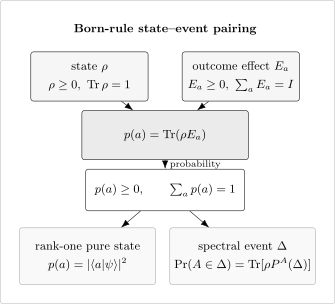
The Born rule pairs a state $\rho$ with an outcome effect $E_a$. Rank-one projectors give squared overlaps, while spectral projectors give probabilities for sets of observable values.

Optional check: why the general formula gives probabilities

General probability checks

The operator conditions are exactly what make $p(a)=\operatorname{Tr}(\rho E_a)$ a probability distribution.

Positivity

Because $\rho$ and $E_a$ are positive,

$$\begin{aligned} p(a) &= \operatorname{Tr}(\rho E_a)\\ &= \operatorname{Tr} \left( \rho^{1/2}E_a\rho^{1/2} \right) \geq0. \end{aligned}$$

The operator inside the final trace is positive. In infinite-dimensional settings, $\rho$ is trace class and each bounded effect satisfies $0\leq E_a\leq I$, so the pairing remains well defined.

Normalization

Completeness of the measurement gives

$$\begin{aligned} \sum_a p(a) &= \sum_a \operatorname{Tr}(\rho E_a)\\ &= \operatorname{Tr} \left( \rho\sum_a E_a \right)\\ &= \operatorname{Tr}\rho = 1. \end{aligned}$$

Upper bound

Since $I-E_a\geq0$,

$$1-p(a) = \operatorname{Tr} \left[ \rho(I-E_a) \right] \geq0.$$

Therefore $0\leq p(a)\leq1$.

Additivity and coarse-graining

If a coarse outcome $S$ combines mutually exclusive fine outcomes $a\in S$, its effect is

$$E_S = \sum_{a\in S}E_a.$$

The corresponding probability is additive:

$$\begin{aligned} p(S) &= \operatorname{Tr}(\rho E_S)\\ &= \sum_{a\in S} \operatorname{Tr}(\rho E_a)\\ &= \sum_{a\in S}p(a). \end{aligned}$$

The additivity applies to mutually exclusive outcomes within one declared measurement. It is not permission to assign a classical joint distribution to arbitrary noncommuting observables.

Rank-One Pure-State Form

Let the outcome ray be represented by a normalized ket $\lvert a\rangle$, with projector

$$\Pi_a = \lvert a\rangle\langle a\rvert.$$

For a normalized pure input,

$$\begin{aligned} p(a\mid\psi) &= \langle\psi\rvert\Pi_a\lvert\psi\rangle\\ &= \langle\psi\rvert a\rangle \langle a\rvert\psi\rangle\\ &= \lvert\langle a\rvert\psi\rangle\rvert^2. \end{aligned}$$

The complex overlap is a probability amplitude; its squared modulus is the probability. Probability Amplitudes develops the rules for composing, adding, and rephasing such amplitudes.

If $\{\lvert a\rangle\}$ is a complete orthonormal basis, then

$$\sum_a \lvert\langle a\rvert\psi\rangle\rvert^2 = 1.$$

The basis must be the eigenbasis or outcome basis of the measurement being performed. Coefficients in an unrelated basis do not directly give the desired outcome probabilities.

Projective Measurements and Degeneracy

A projective measurement is described by projectors $\{P_a\}$ satisfying

$$P_aP_b = \delta_{ab}P_a, \qquad \sum_aP_a = I.$$

The Born probability is

$$p(a) = \operatorname{Tr}(\rho P_a).$$

If the input is pure,

$$p(a) = \lVert P_a\lvert\psi\rangle\rVert^2.$$

For a $d_a$-dimensional outcome subspace with orthonormal basis $\{\lvert a,\alpha\rangle\}$,

$$P_a = \sum_{\alpha=1}^{d_a} \lvert a,\alpha\rangle \langle a,\alpha\rvert,$$

and

$$p(a) = \sum_{\alpha=1}^{d_a} \lvert \langle a,\alpha\rvert\psi\rangle \rvert^2.$$

The sum is independent of the orthonormal basis chosen inside the degenerate subspace. Selecting one arbitrary eigenvector and squaring only its overlap would undercount the outcome probability.

Born Rule for Discrete Spectra owns the step-by-step finite and countable workflow, including degeneracy and normalization checks.

Observables and Spectral Events

A self-adjoint observable $A$ has a projection-valued spectral measure $P^A$. For a measurable set of values $\Delta\subseteq\mathbb R$, the event “the measured value of $A$ lies in $\Delta$” is represented by $P^A(\Delta)$. The Born probability measure is

$$\mu_\rho^A(\Delta) = \operatorname{Tr} \left[ \rho P^A(\Delta) \right].$$

This formulation treats discrete, continuous, and mixed spectra uniformly. It satisfies

$$\mu_\rho^A(\mathbb R) = 1$$

and, for pairwise disjoint measurable sets $\Delta_j$,

$$\mu_\rho^A \left( \bigcup_j\Delta_j \right) = \sum_j \mu_\rho^A(\Delta_j).$$

For a discrete eigenvalue $a$,

$$P^A(\{a\}) = P_a.$$

For a purely continuous distribution, the projector of one exact point often has zero probability even though intervals containing that point can have nonzero probability.

The operator construction belongs to Spectral Decomposition and Spectra. The Born rule uses the resulting spectral events to assign probabilities.

Density Operators and Ensemble Independence

A density operator satisfies

$$\rho\geq0, \qquad \operatorname{Tr}\rho=1.$$

If one preparation procedure is represented as an ensemble

$$\begin{aligned} \rho &= \sum_k w_k \lvert\psi_k\rangle \langle\psi_k\rvert,\\ w_k&\geq0, & \sum_kw_k&=1, \end{aligned}$$

then

$$\begin{aligned} p(a) &= \operatorname{Tr}(\rho E_a)\\ &= \sum_k w_k \langle\psi_k\rvert E_a\lvert\psi_k\rangle. \end{aligned}$$

The probability is affine in the state: classical randomization among preparations randomizes the corresponding quantum probabilities.

The same $\rho$ can have many different pure-state ensemble decompositions. Because the Born probability depends only on $\rho$, all such decompositions are operationally equivalent for measurements on that system. Density Operators owns the state theory and the distinction between mixtures and superpositions.

Continuous Position Measurements

For a pure state with position-space wavefunction

$$\psi(x) = \langle x\rvert\psi\rangle,$$

the ideal position event $x\in\Delta$ has probability

$$\Pr_\psi(x\in\Delta) = \int_\Delta \lvert\psi(x)\rvert^2\,dx.$$

The integrand is a density with respect to $dx$:

$$\Pr_\psi(x\in[x,x+dx]) \approx \lvert\psi(x)\rvert^2dx.$$

For a density operator with position kernel

$$\rho(x,x') = \langle x\rvert\rho\lvert x'\rangle,$$

the same probability is

$$\Pr_\rho(x\in\Delta) = \int_\Delta \rho(x,x)\,dx.$$

An exact value $x_0$ has probability zero for an ordinary absolutely continuous state:

$$\Pr(x=x_0) = 0.$$

This does not mean the density vanishes at $x_0$. Probability requires a set and a measure. Delta normalization, interval probabilities, mixed spectra, and changes of variables are developed in Born Rule for Continuous Spectra.

Generalized Measurements

A positive-operator-valued measure, or POVM, is a collection of effects $\{E_a\}$ with

$$E_a\geq0, \qquad \sum_aE_a=I.$$

Projective measurements are the special case in which

$$E_a^2=E_a, \qquad E_aE_b=0 \quad (a\neq b).$$

General effects need not be idempotent or mutually orthogonal. They can model finite detector resolution, noisy discrimination, indirect measurements, and coarse-grained readouts while retaining the same probability formula:

$$p(a) = \operatorname{Tr}(\rho E_a).$$

The Born-rule page needs this generality to state the probability postulate, but the construction and interpretation of effects belong to POVMs: First Encounter.

For a continuous outcome space $\Omega$, the collection is replaced by a normalized operator-valued measure $E$. A measurable outcome set $\Delta\subseteq\Omega$ has probability

$$p(\Delta) = \operatorname{Tr} \left[ \rho E(\Delta) \right], \qquad E(\Omega)=I.$$

Countable additivity of $E$ on disjoint sets induces countable additivity of the resulting probability measure.

Classical Postprocessing

A detector may first produce a fine outcome $a$ and then report $b$ with classical conditional probability $q(b\mid a)$. The reported effect is

$$F_b = \sum_a q(b\mid a)E_a.$$

The effects remain normalized:

$$\sum_bF_b = \sum_a \left[ \sum_bq(b\mid a) \right] E_a = I.$$

The reported probability is

$$\begin{aligned} p(b) &= \operatorname{Tr}(\rho F_b)\\ &= \sum_a q(b\mid a)p(a). \end{aligned}$$

This is ordinary classical probability processing applied after the quantum state–effect pairing. It should not be confused with coherent addition of quantum amplitudes.

Representation Independence

Changing basis by a unitary $U$ transforms both state and effect:

$$\rho' = U\rho U^\dagger, \qquad E_a' = UE_aU^\dagger.$$

The probability is unchanged:

$$\begin{aligned} \operatorname{Tr}(\rho'E_a') &= \operatorname{Tr} \left( U\rho E_aU^\dagger \right)\\ &= \operatorname{Tr}(\rho E_a). \end{aligned}$$

This is a passive representation change. An active physical transformation of the state while the laboratory measurement remains fixed generally changes the probability. The calculation must distinguish those two situations.

Expectation Values from the Outcome Distribution

For a discrete observable

$$A = \sum_a aP_a,$$

the Born probabilities induce the expectation value

$$\begin{aligned} \mathbb E_\rho[A] &= \sum_a a\,p(a)\\ &= \sum_a a\operatorname{Tr}(\rho P_a)\\ &= \operatorname{Tr}(\rho A). \end{aligned}$$

The analogous spectral integral applies to continuous observables when the state lies in the required domain. The statistical interpretation, unbounded operator caveats, and worked calculations belong to Expectation Values.

Worked Example: Qubit Along an Arbitrary Axis

Write a qubit state in Bloch form,

$$\rho = \frac12 \left( I+\mathbf r\cdot\boldsymbol\sigma \right), \qquad \lVert\mathbf r\rVert\leq1.$$

A sharp spin measurement along the unit vector $\mathbf n$ has projectors

$$P_\pm = \frac12 \left( I\pm\mathbf n\cdot\boldsymbol\sigma \right).$$

Using

$$\begin{aligned} \operatorname{Tr}I&=2, & \operatorname{Tr}\sigma_i&=0,\\ \operatorname{Tr}(\sigma_i\sigma_j) &= 2\delta_{ij}, \end{aligned}$$

the Born rule gives

$$\begin{aligned} p(\pm) &= \operatorname{Tr}(\rho P_\pm)\\ &= \frac12 \left( 1\pm\mathbf r\cdot\mathbf n \right). \end{aligned}$$

The probabilities are nonnegative because $\lvert\mathbf r\cdot\mathbf n\rvert\leq1$, and they sum to one. For a pure state aligned with $\mathbf n$, the $+$ outcome is certain. For the maximally mixed state $\mathbf r=\mathbf0$, both outcomes have probability $1/2$ for every axis.

The geometric state description is developed in Bloch Sphere.

Worked Example: A Degenerate Energy Outcome

Let an energy eigenspace with energy $E$ be spanned by $\lvert E,1\rangle$ and $\lvert E,2\rangle$. Its projector is

$$P_E = \lvert E,1\rangle\langle E,1\rvert + \lvert E,2\rangle\langle E,2\rvert.$$

For

$$\lvert\psi\rangle = c_0\lvert E_0\rangle + c_1\lvert E,1\rangle + c_2\lvert E,2\rangle,$$

the probability of measuring the value $E$ is

$$p(E) = \lvert c_1\rvert^2 + \lvert c_2\rvert^2.$$

The apparatus resolves the eigenvalue but not an arbitrary basis label inside its eigenspace. Summing the two orthogonal components is therefore essential.

Probability Does Not Specify State Update

Suppose a measurement outcome $a$ is implemented by an operator $M_a$ with

$$E_a = M_a^\dagger M_a.$$

Then

$$\begin{aligned} p(a) &= \operatorname{Tr} \left( M_a\rho M_a^\dagger \right)\\ &= \operatorname{Tr}(\rho E_a). \end{aligned}$$

If the outcome occurs, one possible conditional update is

$$\rho \longmapsto \rho_a' = \frac{ M_a\rho M_a^\dagger }{ p(a) }.$$

But the effect $E_a$ does not uniquely determine $M_a$. For any unitary $V_a$,

$$N_a = V_aM_a$$

has the same effect,

$$N_a^\dagger N_a = E_a,$$

and therefore the same Born probability, while generally producing a different conditional state.

The Born rule determines outcome statistics. A complete state-update rule requires an instrument or an explicit measurement model. See Projective Measurement, State Update Rule, and Generalized Measurements Overview.

What the Rule Assumes

At this level, the Born rule assumes the standard quantum framework:

• preparations are represented by normalized state vectors or positive trace-one density operators;
• measurement events are represented by projectors, spectral projectors, or more general effects;
• the state and measurement refer to the same system and Hilbert space;
• outcome probabilities are assigned by the state–effect pairing;
• the measurement is complete, so its effects sum to the identity.

It also assumes that the state and measurement model have already been chosen. Connecting laboratory controls, detector calibration, and data processing to $\rho$ and $\{E_a\}$ is a modeling and inference task, not something the formula performs automatically.

Status of Derivations and Reconstruction Theorems

In standard presentations of quantum mechanics, the Born rule is a postulate. Mathematical reconstruction results can show that the trace form is forced once particular structural assumptions are accepted.

For example, Gleason’s theorem starts with an additive probability assignment to Hilbert-space projectors and, in Hilbert spaces of dimension at least three, obtains a density-operator representation

$$\mu(P) = \operatorname{Tr}(\rho P).$$

The theorem is profound, but it is not an assumption-free derivation of quantum probability. It presupposes the Hilbert-space event structure, additivity, and a context-independent assignment to projectors. The original dimension restriction and the assumptions of POVM-based extensions must also be stated. See Gleason’s Theorem for the theorem-level treatment.

Interpretive, decision-theoretic, envariance-based, and operational reconstruction programs ask different questions and use different assumptions. They should not be compressed into the formal probability rule or advertised as derivations from nothing.

What the Rule Does Not Explain

By itself, the Born rule does not determine:

• why one individual outcome occurs in a particular run;
• whether probabilities are objective chances, rational credences, branch weights, or something else;
• whether observables possess values before measurement;
• the ontology of the wavefunction or density operator;
• whether and how a physical collapse occurs;
• which interpretation of quantum mechanics is correct;
• why the Hilbert-space formalism is realized in nature.

These are foundational questions. The formal rule should be stated precisely before interpretive claims are layered on top of it. What the Postulates Do Not Say gives the broader boundary.

A Reliable Calculation Workflow

1. Specify the state. Use a normalized $\lvert\psi\rangle$ or a positive trace-one $\rho$.
2. Specify the measurement. Identify the complete PVM or POVM, not only an informal observable name.
3. Identify the event. Use the projector, effect, or spectral set matching the outcome being asked about.
4. Choose the appropriate form. Use a squared overlap only for a rank-one pure-state event; otherwise use a projector norm or trace.
5. Coarse-grain deliberately. Sum effects or probabilities only for mutually exclusive outcomes of the same measurement.
6. Check the distribution. Verify nonnegativity and unit total probability.
7. Separate prediction from update. Do not infer a post-measurement state from the probability formula alone.

Diagnostic Checks

Normalization

$$\sum_a p(a) = 1$$

for an exhaustive discrete measurement, or

$$\mu_\rho^A(\mathbb R) = 1$$

for a spectral probability measure.

Positivity

$$p(a)\geq0$$

for every physical state. A proposed effect that produces a negative value for some state is not positive and cannot represent an outcome.

Certain and impossible events

$$\operatorname{Tr}(\rho I) = 1, \qquad \operatorname{Tr}(\rho\,0) = 0.$$

Basis invariance

$$\operatorname{Tr} \left( U\rho U^\dagger UE_aU^\dagger \right) = \operatorname{Tr}(\rho E_a).$$

Coarse-graining

$$p(S) = \sum_{a\in S}p(a)$$

only when $S$ is a union of mutually exclusive outcomes within the declared measurement.

Common Mistakes

• Applying the squared-overlap formula without naming the measurement basis.
• Using one eigenvector instead of the full projector for a degenerate eigenvalue.
• Treating $\lvert\psi(x)\rvert^2$ as a point probability rather than a density relative to $dx$.
• Forgetting to normalize the state or to complete the measurement effects.
• Assuming every POVM effect is a projector.
• Computing $\lvert\operatorname{Tr}(\rho E_a)\rvert^2$ instead of $\operatorname{Tr}(\rho E_a)$.
• Transforming the state to a new basis while leaving the measurement effect in the old basis.
• Adding probabilities for coherent alternatives before the measurement has made them mutually exclusive.
• Treating a POVM effect as though it uniquely determined the conditional post-measurement state.
• Reading the Born rule as a claim that outcomes reveal pre-existing classical values.
• Calling a reconstruction theorem an assumption-free derivation of the rule.

Canonical Boundaries and Cross-Links

• Probability Amplitudes owns coherent addition, composition, and phase conventions before the squared-modulus step.
• Born Rule for Discrete Spectra owns practical finite and countable calculations.
• Born Rule for Continuous Spectra owns densities, intervals, generalized eigenstates, and mixed spectra.
• Expectation Values owns moments of the induced outcome distribution.
• Projectors and Spectral Decomposition own the operator structures representing sharp events.
• POVMs: First Encounter owns effects and generalized-measurement examples.
• State Update Rule owns conditional post-measurement states and instruments.

References

• M. Born, “Zur Quantenmechanik der Stoßvorgänge”, Zeitschrift für Physik 37, 863–867 (1926). The paper introduced the statistical interpretation of scattering amplitudes.
• P. Busch, P. J. Lahti, J.-P. Pellonpää, and K. Ylinen, Quantum Measurement, Springer, 2016. Gives a modern treatment of effects, POVMs, observables, and instruments.
• P. A. M. Dirac, The Principles of Quantum Mechanics, 4th ed., Oxford University Press, 1958. Gives the transformation-function and projection viewpoints in bra-ket language.
• A. M. Gleason, “Measures on the Closed Subspaces of a Hilbert Space”, Journal of Mathematics and Mechanics 6, 885–893 (1957).
• A. S. Holevo, Probabilistic and Statistical Aspects of Quantum Theory, North-Holland, 1982. Develops quantum probability and generalized measurements systematically.
• A. Peres, Quantum Theory: Concepts and Methods, Kluwer, 1995. Emphasizes operational distinctions among preparations, measurements, and outcomes.
• J. J. Sakurai and J. Napolitano, Modern Quantum Mechanics, 3rd ed., Cambridge University Press, 2020. Provides standard pure-state, projector, and density-matrix formulations.
• J. von Neumann, Mathematical Foundations of Quantum Mechanics, Princeton University Press, English translation, 1955. Develops the projection and density-operator probability framework.

Exercises

Exercise 1: Rank-one outcome

Let

$$\lvert\psi\rangle = \frac{ 2\lvert0\rangle+i\lvert1\rangle }{\sqrt5}, \qquad \lvert+\rangle = \frac{ \lvert0\rangle+\lvert1\rangle }{\sqrt2}.$$

Find the probability of the $+$ outcome.

Solution

The transition amplitude is

$$\langle+\rvert\psi\rangle = \frac{2+i}{\sqrt{10}}.$$

Therefore

$$\begin{aligned} p(+) &= \left\lvert \frac{2+i}{\sqrt{10}} \right\rvert^2\\ &= \frac{4+1}{10} = \frac12. \end{aligned}$$

Exercise 2: Degenerate projector

In a three-dimensional orthonormal basis, define

$$P = \lvert1\rangle\langle1\rvert + \lvert2\rangle\langle2\rvert$$

and

$$\lvert\psi\rangle = \frac{ \lvert0\rangle +i\lvert1\rangle +2\lvert2\rangle }{\sqrt6}.$$

Find the probability of the outcome represented by $P$.

Solution

The projected branch is

$$P\lvert\psi\rangle = \frac{ i\lvert1\rangle +2\lvert2\rangle }{\sqrt6}.$$

Its squared norm is

$$p(P) = \frac16+\frac46 = \frac56.$$

The two components are summed because the projector represents one degenerate outcome.

Exercise 3: Mixed state in another basis

Let

$$\rho = \frac34 \lvert0\rangle\langle0\rvert + \frac14 \lvert1\rangle\langle1\rvert.$$

Compute the probabilities for a measurement in the $\{\lvert+\rangle,\lvert-\rangle\}$ basis.

Solution

For either sign,

$$\lvert\langle\pm\rvert0\rangle\rvert^2 = \lvert\langle\pm\rvert1\rangle\rvert^2 = \frac12.$$

Hence

$$\begin{aligned} p(\pm) &= \operatorname{Tr} \left( \rho\lvert\pm\rangle\langle\pm\rvert \right)\\ &= \frac34\frac12 + \frac14\frac12 = \frac12. \end{aligned}$$

The unequal populations in the computational basis do not produce unequal probabilities in this complementary basis.

Exercise 4: Probability axioms from a POVM

Let $\rho$ be a density operator and let $\{E_a\}$ satisfy $E_a\geq0$ and $\sum_aE_a=I$. Prove that $p(a)=\operatorname{Tr}(\rho E_a)$ is nonnegative, bounded by one, and normalized.

Solution

Positivity follows from

$$p(a) = \operatorname{Tr} \left( \rho^{1/2}E_a\rho^{1/2} \right) \geq0.$$

Because $I-E_a$ is also positive,

$$1-p(a) = \operatorname{Tr} \left[ \rho(I-E_a) \right] \geq0,$$

so $p(a)\leq1$. Finally,

$$\sum_ap(a) = \operatorname{Tr} \left( \rho\sum_aE_a \right) = \operatorname{Tr}\rho = 1.$$

Exercise 5: Bloch-vector probability

A qubit has Bloch vector

$$\mathbf r = (0,0,r), \qquad -1\leq r\leq1.$$

A sharp measurement axis $\mathbf n$ makes polar angle $\theta$ with the positive $z$ axis. Find $p(+)$ and $p(-)$.

Solution

The dot product is

$$\mathbf r\cdot\mathbf n = r\cos\theta.$$

Using the qubit Born formula,

$$p(\pm) = \frac12 \left( 1\pm r\cos\theta \right).$$

The probabilities sum to one. For $r=1$ and $\theta=0$, the $+$ outcome is certain; for $r=0$, both outcomes have probability $1/2$ for every axis.

Exercise 6: Position in half a box

A normalized particle-in-a-box state on $0<x<L$ is

$$\psi(x) = \sqrt{\frac2L} \sin\frac{\pi x}{L}.$$

Find the probability of detecting the particle in the left half, $0<x<L/2$.

Solution

Writing $p_L=\Pr(0<x<L/2)$, the interval probability is

$$\begin{aligned} p_L &= \frac2L \int_0^{L/2} \sin^2\frac{\pi x}{L}\,dx\\ &= \frac1L \left[ x - \frac{L}{2\pi} \sin\frac{2\pi x}{L} \right]_0^{L/2}\\ &= \frac12. \end{aligned}$$

The result also follows from the symmetry of $\lvert\psi(x)\rvert^2$ about $x=L/2$.

Exercise 7: Basis invariance

Show directly that a simultaneous unitary representation change

$$\rho' = U\rho U^\dagger, \qquad E_a' = UE_aU^\dagger$$

leaves the Born probability unchanged.

Solution

Multiply the represented operators:

$$\rho'E_a' = U\rho U^\dagger UE_aU^\dagger = U\rho E_aU^\dagger.$$

Cyclicity of the trace and $U^\dagger U=I$ give

$$\begin{aligned} \operatorname{Tr}(\rho'E_a') &= \operatorname{Tr} \left( U\rho E_aU^\dagger \right)\\ &= \operatorname{Tr} \left( \rho E_aU^\dagger U \right)\\ &= \operatorname{Tr}(\rho E_a). \end{aligned}$$

Exercise 8: Same probabilities, different updates

For the computational-basis effects

$$E_0 = \lvert0\rangle\langle0\rvert, \qquad E_1 = \lvert1\rangle\langle1\rvert,$$

compare the measurement operators

$$M_0=E_0, \qquad M_1=E_1$$

with

$$N_0 = \lvert+\rangle\langle0\rvert, \qquad N_1 = \lvert+\rangle\langle1\rvert.$$

Show that they give the same outcome probabilities but different conditional states.

Solution

For the first implementation,

$$M_a^\dagger M_a = E_a.$$

For the second,

$$\begin{aligned} N_0^\dagger N_0 &= \lvert0\rangle \langle+\rvert+\rangle \langle0\rvert = E_0,\\ N_1^\dagger N_1 &= \lvert1\rangle \langle+\rvert+\rangle \langle1\rvert = E_1. \end{aligned}$$

Both implementations therefore give

$$p(a) = \operatorname{Tr}(\rho E_a).$$

For any outcome with nonzero probability, the $M_a$ implementation prepares the corresponding computational-basis state $\lvert a\rangle$. The $N_a$ implementation prepares $\lvert+\rangle$ for either outcome. The statistics are the same, but the conditional states differ.