Variance and Standard Deviation

The variance of an observable quantifies the intrinsic spread of its Born-rule measurement outcomes about their expectation value. For a state $\rho$ and a self-adjoint observable $A$, define the centered observable

$$\delta_\rho A \equiv A-\langle A\rangle_\rho I.$$

The variance and standard deviation are

$$\operatorname{Var}_\rho(A) \equiv (\Delta_\rho A)^2 = \left\langle(\delta_\rho A)^2\right\rangle_\rho,$$

and

$$\Delta_\rho A = \sqrt{\operatorname{Var}_\rho(A)}.$$

The standard deviation has the same physical units as $A$; the variance has squared units. Neither quantity is, by itself, an apparatus error or a claim about measurement disturbance. It is a property of the observable’s outcome distribution in the specified state.

This page develops the quantum interpretation, operator forms, domain conditions, and examples. The generic probability theory belongs at Variance and Covariance, while the inequalities relating spreads of two observables belong at General Uncertainty Relations.

Required background. Expectation Values supplies the first and second moments used here.

Helpful background. Functions of Operators supplies squared and centered observables.

Spread around the expectation

Let $\mu_\rho^A$ be the Born probability measure of $A$. If its second moment is finite, then

$$\operatorname{Var}_\rho(A) = \int_{\mathbb R} (\lambda-\langle A\rangle_\rho)^2 \,d\mu_\rho^A(\lambda).$$

The integrand is nonnegative and measures the squared displacement of each outcome from the mean. Outcomes twice as far from the mean contribute four times as much, so variance is especially sensitive to tails and outliers.

Two distributions can have the same expectation but very different spreads.

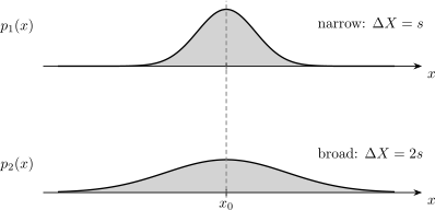
Both distributions are centered at $x_0$, but the lower distribution has the larger standard deviation. A mean identifies a center; it does not determine the width or shape of the outcome law.

Variance is therefore information beyond the expectation value. It still does not determine the full distribution: laws with different skewness, tails, or multiple peaks can share both mean and variance.

Equivalent moment formula

Expanding the centered square gives

$$\begin{aligned} \operatorname{Var}_\rho(A) &= \left\langle A^2-2\langle A\rangle_\rho A +\langle A\rangle_\rho^2 I \right\rangle_\rho\\ &= \langle A^2\rangle_\rho - \langle A\rangle_\rho^2. \end{aligned}$$

Thus

$$\Delta_\rho A = \sqrt{ \langle A^2\rangle_\rho - \langle A\rangle_\rho^2 }.$$

The central-moment form and raw-moment form are mathematically equivalent when the moments exist. The central form is often numerically safer because $\langle A^2\rangle$ and $\langle A\rangle^2$ can be large, nearly equal numbers whose subtraction loses floating-point precision.

Discrete outcomes

For a discrete spectral decomposition

$$A = \sum_a aP_a,$$

the probability of outcome $a$ is

$$p_\rho(a) = \operatorname{Tr}(\rho P_a).$$

The variance is the ordinary discrete second central moment:

$$\operatorname{Var}_\rho(A) = \sum_a (a-\langle A\rangle_\rho)^2 p_\rho(a).$$

Equivalently,

$$\operatorname{Var}_\rho(A) = \sum_a a^2p_\rho(a) - \left[ \sum_a ap_\rho(a) \right]^2.$$

Degeneracy is already included because $P_a$ projects onto the entire eigenspace. The probabilities themselves are developed at Born Rule for Discrete Spectra.

Continuous and mixed outcomes

If the spectral probability measure has density $p_A(\lambda)$, then

$$\operatorname{Var}_\rho(A) = \int_{-\infty}^{\infty} (\lambda-\langle A\rangle_\rho)^2 p_A(\lambda)\,d\lambda.$$

For one-dimensional position,

$$(\Delta X)^2 = \int_{-\infty}^{\infty} (x-\langle X\rangle)^2 |\psi(x)|^2\,dx.$$

For a mixed spectral law with atomic weights $w_n$ at $a_n$ and continuous density $p_{\mathrm{ac}}(\lambda)$,

$$\begin{aligned} \operatorname{Var}_\rho(A) &= \sum_n(a_n-\langle A\rangle_\rho)^2w_n\\ &\quad+ \int_{\mathbb R} (\lambda-\langle A\rangle_\rho)^2 p_{\mathrm{ac}}(\lambda)\,d\lambda. \end{aligned}$$

The density, atoms, and coordinate-measure rules are treated at Born Rule for Continuous Spectra.

Pure-state norm form

For a normalized pure state, define

$$|f_A\rangle \equiv (A-\langle A\rangle_\psi I)|\psi\rangle.$$

Then

$$\begin{aligned} (\Delta_\psi A)^2 &= \langle f_A|f_A\rangle\\ &= \left\| (A-\langle A\rangle_\psi I)|\psi\rangle \right\|^2. \end{aligned}$$

This form immediately proves

$$(\Delta_\psi A)^2\ge0.$$

It also supplies the vectors used in the Cauchy–Schwarz derivation of quantum uncertainty relations. The norm form is more than a proof trick: for unbounded operators, it expresses the second spectral moment without unnecessarily requiring $A^2|\psi\rangle$ to exist as a vector.

Domain and finite-moment conditions

For a pure state and self-adjoint $A$, a finite second moment requires

$$\int_{\mathbb R}\lambda^2 \,d\mu_\psi^A(\lambda)<\infty.$$

This is equivalent to

$$|\psi\rangle\in D(A),$$

and then

$$\int_{\mathbb R}\lambda^2 \,d\mu_\psi^A(\lambda) = \|A\psi\|^2.$$

The notation $\langle A^2\rangle$ in a variance formula should therefore be understood as this second spectral moment or quadratic form. Requiring the operator expression $A^2|\psi\rangle$ would demand $|\psi\rangle\in D(A^2)$, a stronger condition that is not needed merely to define the variance.

A normalized state can have a finite mean but infinite second moment. In that case the standard deviation is infinite, and formulas that assume a finite variance, such as the usual standard error of a sample mean, do not apply.

Density-operator formula

For a density operator $\rho$ and a bounded observable $A$,

$$\operatorname{Var}_\rho(A) = \operatorname{Tr}(\rho A^2) - \left[ \operatorname{Tr}(\rho A) \right]^2.$$

Equivalently,

$$\operatorname{Var}_\rho(A) = \operatorname{Tr}\!\left[ \rho(\delta_\rho A)^2 \right].$$

For unbounded $A$, these traces require the corresponding finite-moment and domain conditions. The full trace formalism is at Trace Rule for Expectation Values.

Quantum and mixing contributions

Suppose a preparation is represented as

$$\rho = \sum_j q_j\rho_j, \qquad q_j\ge0, \qquad \sum_jq_j=1.$$

Let

$$\begin{aligned} \mu_j &= \operatorname{Tr}(\rho_jA),\\ \mu &= \operatorname{Tr}(\rho A) = \sum_jq_j\mu_j. \end{aligned}$$

The law of total variance gives

$$\begin{aligned} \operatorname{Var}_\rho(A) &= \sum_jq_j\operatorname{Var}_{\rho_j}(A)\\ &\quad+ \sum_jq_j(\mu_j-\mu)^2. \end{aligned}$$

The first term averages the within-component quantum spreads; the second is the spread of the component means. This decomposition depends on the chosen ensemble realization of $\rho$, whereas the total variance depends only on $\rho$. Because a density operator generally has many ensemble decompositions, the two terms are not intrinsic state invariants separately.

Affine transformations and units

For real $\alpha$ and $\beta$,

$$\operatorname{Var}_\rho(\alpha A+\beta I) = \alpha^2\operatorname{Var}_\rho(A),$$

and

$$\Delta_\rho(\alpha A+\beta I) = |\alpha|\Delta_\rho A.$$

Adding a constant shifts every outcome and the mean by the same amount, so it does not change the spread. Multiplying the observable rescales every deviation.

For example, if $S_z=(\hbar/2)\sigma_z$, then

$$\Delta S_z = \frac{\hbar}{2}\Delta\sigma_z.$$

This scaling is also a dimensional check: standard deviation carries the observable’s units, while variance carries their square.

Two-outcome formula

Let $A$ have outcomes $a_-$ and $a_+$ with probabilities $1-p$ and $p$. Its expectation is

$$\mu = (1-p)a_-+pa_+.$$

Direct calculation gives

$$\operatorname{Var}(A) = p(1-p)(a_+-a_-)^2.$$

The variance vanishes at $p=0$ or $p=1$, when the outcome is certain, and is maximal at $p=1/2$. For fixed outcomes,

$$\operatorname{Var}(A) \le \frac{(a_+-a_-)^2}{4}.$$

This compact formula covers projective measurements of any two-level observable.

Example: spin one-half

Consider

$$|\psi\rangle = \cos\frac{\theta}{2}|+z\rangle + e^{i\phi}\sin\frac{\theta}{2}|-z\rangle.$$

For $\sigma_z$,

$$\langle\sigma_z\rangle = \cos\theta, \qquad \langle\sigma_z^2\rangle=1.$$

Therefore

$$\begin{aligned} (\Delta\sigma_z)^2 &= 1-\cos^2\theta = \sin^2\theta,\\ \Delta\sigma_z &= |\sin\theta|. \end{aligned}$$

For the physical spin component,

$$\Delta S_z = \frac{\hbar}{2}|\sin\theta|.$$

The phase $\phi$ does not affect the $z$-outcome probabilities, but it affects spreads of spin components along other directions. The $S_z$ eigenstates have zero $S_z$ variance, while an equatorial state has the maximal value $\hbar^2/4$.

Qubit form for arbitrary direction

Let

$$\rho = \frac12(I+\mathbf r\cdot\boldsymbol\sigma)$$

and measure

$$A = \mathbf n\cdot\boldsymbol\sigma, \qquad |\mathbf n|=1.$$

Because $A^2=I$,

$$\operatorname{Var}_\rho(A) = 1-(\mathbf r\cdot\mathbf n)^2.$$

A pure state with $\mathbf r=\pm\mathbf n$ has a definite outcome and zero variance. The maximally mixed state has $\mathbf r=0$ and unit variance for every spin direction, even though every spin expectation vanishes.

Example: Gaussian position spread

Consider the normalized position density

$$p_X(x) = \frac{1}{\sqrt{2\pi}s} \exp\!\left[ -\frac{(x-x_0)^2}{2s^2} \right].$$

Its first two raw moments are

$$\langle X\rangle=x_0, \qquad \langle X^2\rangle=x_0^2+s^2.$$

Consequently,

$$\operatorname{Var}(X)=s^2, \qquad \Delta X=s.$$

Wavefunctions are often parameterized with symbols called “width” that differ by factors of $2$ or $\sqrt2$. Computing the variance identifies the physical standard deviation independent of naming convention.

Zero variance and definite values

For a pure state, the norm form implies

$$\Delta_\psi A=0$$

if and only if

$$(A-\langle A\rangle_\psi I)|\psi\rangle=0.$$

Thus the state is an eigenvector of $A$ with eigenvalue $\langle A\rangle_\psi$.

For a mixed state, zero variance means that the support of $\rho$ lies entirely inside one eigenspace of $A$:

$$\operatorname{supp}(\rho) \subseteq \ker(A-\langle A\rangle_\rho I).$$

The state may still be mixed within a degenerate eigenspace. Zero variance therefore implies a definite measurement value, not necessarily a pure state.

Spectral bounds on variance

If the spectrum relevant to the measurement lies in $[m,M]$, then the Bhatia–Davis bound gives

$$\operatorname{Var}_\rho(A) \le (M-\langle A\rangle_\rho) (\langle A\rangle_\rho-m).$$

Since the product on the right is at most $(M-m)^2/4$,

$$\operatorname{Var}_\rho(A) \le \frac{(M-m)^2}{4}.$$

For a qubit observable with outcomes $\pm1$, this yields $\operatorname{Var}(A)\le1$. Such bounds are strong sanity checks for analytic and numerical calculations.

Estimating variance from data

For $N$ independent outcomes $a_1,\ldots,a_N$, define the sample mean

$$\overline a = \frac1N\sum_{j=1}^N a_j.$$

The usual unbiased estimator of the population variance is

$$s_A^2 = \frac{1}{N-1} \sum_{j=1}^N(a_j-\overline a)^2.$$

The factor $N-1$ corrects the bias introduced by estimating the mean from the same data. The quantum prediction $\operatorname{Var}_\rho(A)$ is the population quantity that repeated experiments estimate; one should not confuse it with a particular finite-sample value $s_A^2$.

When the variance is finite, the standard deviation of the sample mean is

$$\Delta\overline A_N = \frac{\Delta A}{\sqrt N}.$$

This describes independent statistical fluctuations. Correlated trials, drifting preparations, and detector systematics require a more complete error model.

Intrinsic spread and detector noise

Suppose a recorded value has the additive form

$$Y=A+N,$$

where the ideal quantum outcome $A$ and detector noise $N$ are independent and have finite variances. Then

$$\operatorname{Var}(Y) = \operatorname{Var}(A) + \operatorname{Var}(N).$$

This decomposition is a model assumption, not a universal measurement law. Correlated noise, nonlinear response, and general POVMs require different treatments. It nevertheless illustrates why intrinsic quantum spread and instrumental resolution should be specified separately.

Numerical stability

The identity

$$\operatorname{Var}(A) = \langle A^2\rangle-\langle A\rangle^2$$

can suffer catastrophic cancellation when both terms are large compared with their difference. In numerical work, prefer a centered calculation such as

$$\operatorname{Var}_\psi(A) = \left\| (A-\langle A\rangle_\psi I)|\psi\rangle \right\|^2$$

or a stable online variance algorithm for sampled data. A tiny negative result at the level of floating-point roundoff should be diagnosed and clipped only after verifying normalization and Hermiticity; a materially negative variance signals an error.

Bridge to uncertainty relations

For two observables, define centered-state vectors

$$|f_A\rangle = \delta_\rho A|\psi\rangle, \qquad |f_B\rangle = \delta_\rho B|\psi\rangle$$

in the pure-state case. Their norms are $\Delta A$ and $\Delta B$. Cauchy–Schwarz therefore constrains the product of the two standard deviations. Separating commutator and anticommutator contributions leads to the Robertson and Schrödinger uncertainty relations.

The familiar bound

$$\Delta A\,\Delta B \ge \frac12 \left| \langle[A,B]\rangle \right|$$

concerns outcome-distribution spreads in one state. It is not, by itself, a statement about detector precision or how one measurement disturbs another. The derivation and equality conditions are canonical at General Uncertainty Relations.

Common mistakes

Treating spread as apparatus error

$\Delta A$ is the standard deviation of the ideal Born distribution. Detector noise and calibration uncertainty are separate contributions unless a model explicitly combines them.

Equating zero mean with zero spread

A distribution symmetric about zero can have $\langle A\rangle=0$ and a large variance. The maximally mixed qubit has zero mean spin in every direction and maximal variance for every Pauli measurement.

Forgetting the square on the mean

The identity is

$$\operatorname{Var}(A) = \langle A^2\rangle-\langle A\rangle^2,$$

not $\langle A^2\rangle-\langle A\rangle$.

Squaring matrix elements instead of the operator

$A^2$ means the operator product $AA$, or the spectral function $\lambda\mapsto\lambda^2$. It does not mean squaring each matrix entry.

Ignoring units

$\Delta A$ has the units of $A$; $\operatorname{Var}(A)$ has squared units. Comparing a variance directly to an unsquared physical scale is dimensionally wrong.

Assuming normalization implies finite variance

A normalized Born distribution can have heavy enough tails that its second moment diverges. Check convergence and operator domains for unbounded observables.

Overinterpreting mean and variance

Two moments do not determine the full outcome distribution. Multimodality and rare-event tails can be invisible in a mean-and-standard-deviation summary.

Summary

The variance of $A$ in a state $\rho$ is the second central moment of its Born distribution:

$$\operatorname{Var}_\rho(A) = \int_{\mathbb R} (\lambda-\langle A\rangle_\rho)^2 \,d\mu_\rho^A(\lambda).$$

Equivalent operator notation is

$$\operatorname{Var}_\rho(A) = \langle A^2\rangle_\rho - \langle A\rangle_\rho^2,$$

with the second moment interpreted through the spectral quadratic form when $A$ is unbounded. The standard deviation $\Delta_\rho A$ is nonnegative, has the units of the observable, vanishes exactly for a definite outcome, and provides the norm entering uncertainty relations. Finite variance is an additional condition beyond state normalization.

References

• L. E. Ballentine, Quantum Mechanics: A Modern Development, 2nd ed., World Scientific, 2014, Chapters 2–3.
• R. Bhatia and C. Davis, “A Better Bound on the Variance,” American Mathematical Monthly 107, 353–357 (2000).
• B. C. Hall, Quantum Theory for Mathematicians, Springer, 2013, Chapters 7–10.
• M. Reed and B. Simon, Methods of Modern Mathematical Physics, Vol. I: Functional Analysis, revised and enlarged ed., Academic Press, 1980, Sections VII.1–VII.3 and VIII.3.
• J. J. Sakurai and J. Napolitano, Modern Quantum Mechanics, 3rd ed., Cambridge University Press, 2020, Chapters 1–2.
• R. Shankar, Principles of Quantum Mechanics, 2nd ed., Springer, 1994, Chapters 1 and 4.
• J. von Neumann, Mathematical Foundations of Quantum Mechanics, Princeton University Press, 1955, Chapters II–III.

Exercises

1. Spin variance from Born probabilities

Let $A=\sigma_z$ and

$$|\psi\rangle = \frac{2|+z\rangle+i|-z\rangle}{\sqrt5}.$$

Compute $\langle A\rangle$, $\operatorname{Var}(A)$, and $\Delta A$.

Solution

The probabilities of $+1$ and $-1$ are $4/5$ and $1/5$. Hence

$$\langle A\rangle = \frac45-\frac15 = \frac35.$$

Since $A^2=I$,

$$\begin{aligned} \operatorname{Var}(A) &= 1-\left(\frac35\right)^2 = \frac{16}{25},\\ \Delta A &= \frac45. \end{aligned}$$

2. General two-outcome variance

An observable returns $a_-$ with probability $1-p$ and $a_+$ with probability $p$. Derive

$$\operatorname{Var}(A) = p(1-p)(a_+-a_-)^2$$

and find the probability $p$ that maximizes it.

Solution

The mean is $\mu=(1-p)a_-+pa_+$. The deviations are

$$a_--\mu = -p(a_+-a_-)$$

and

$$a_+-\mu = (1-p)(a_+-a_-).$$

Therefore

$$\begin{aligned} \operatorname{Var}(A) &= (1-p)p^2(a_+-a_-)^2\\ &\quad+ p(1-p)^2(a_+-a_-)^2\\ &= p(1-p)(a_+-a_-)^2. \end{aligned}$$

The factor $p(1-p)$ is maximal at $p=1/2$, where it equals $1/4$.

3. Gaussian position distribution

Suppose

$$p_X(x) = \frac{1}{\sqrt{2\pi}s} e^{-(x-x_0)^2/(2s^2)}.$$

Given $\langle X\rangle=x_0$ and $\langle X^2\rangle=x_0^2+s^2$, compute the variance after the shifted observable $Y=3X-2L$ is introduced, where $L$ has units of length.

Solution

First,

$$\operatorname{Var}(X) = (x_0^2+s^2)-x_0^2 =s^2.$$

The constant shift does not affect variance, while multiplication by $3$ multiplies it by $9$:

$$\operatorname{Var}(Y)=9s^2, \qquad \Delta Y=3s.$$

4. Zero variance for a mixed state

Let $A$ have a degenerate eigenvalue $a$ with orthonormal eigenvectors $|a,1\rangle$ and $|a,2\rangle$. Consider

$$\rho = q|a,1\rangle\langle a,1| + (1-q)|a,2\rangle\langle a,2|.$$

Compute the variance of $A$ and explain why zero variance does not imply that $\rho$ is pure.

Solution

Every state in the support of $\rho$ has the same $A$ outcome $a$. Therefore

$$\langle A\rangle_\rho=a, \qquad \langle A^2\rangle_\rho=a^2,$$

and

$$\operatorname{Var}_\rho(A)=0.$$

For $0<q<1$, the density operator is mixed, but its support lies entirely in one degenerate eigenspace. The observable cannot distinguish mixtures within that eigenspace.

5. Total variance of a preparation mixture

Two preparation procedures are selected with probabilities $q$ and $1-q$. Their outcome means are $\mu_1$ and $\mu_2$, and their variances are $v_1$ and $v_2$. Derive the total variance.

Solution

The total mean is

$$\mu=q\mu_1+(1-q)\mu_2.$$

The law of total variance gives

$$\begin{aligned} v &= qv_1+(1-q)v_2\\ &\quad+ q(\mu_1-\mu)^2 +(1-q)(\mu_2-\mu)^2. \end{aligned}$$

For two components, the between-means term simplifies to

$$q(1-q)(\mu_1-\mu_2)^2.$$

Thus

$$\begin{aligned} v &= qv_1+(1-q)v_2\\ &\quad+ q(1-q)(\mu_1-\mu_2)^2. \end{aligned}$$

6. Finite mean and infinite variance

Consider the even density

$$p(x)=\frac{1}{(1+|x|)^3}.$$

Verify normalization, show that $\langle X\rangle=0$ exists, and show that the variance diverges.

Solution

Normalization follows from

$$\int_{-\infty}^{\infty}p(x)\,dx = 2\int_0^\infty\frac{dx}{(1+x)^3} =1.$$

The absolute first moment is finite:

$$\mathbb E[|X|] = 2\int_0^\infty\frac{x}{(1+x)^3}\,dx =1.$$

Hence evenness legitimately gives $\langle X\rangle=0$. But

$$\langle X^2\rangle = 2\int_0^\infty\frac{x^2}{(1+x)^3}\,dx$$

diverges logarithmically because the integrand behaves as $1/x$ at large $x$. The mean exists, but the variance is infinite.

7. Qubit variance in Bloch form

For

$$\rho=\frac12(I+\mathbf r\cdot\boldsymbol\sigma)$$

and $A=\mathbf n\cdot\boldsymbol\sigma$ with $|\mathbf n|=1$, derive the variance. Evaluate it for the maximally mixed state.

Solution

The Pauli algebra gives $A^2=I$, while

$$\langle A\rangle_\rho = \mathbf r\cdot\mathbf n.$$

Therefore

$$\operatorname{Var}_\rho(A) = 1-(\mathbf r\cdot\mathbf n)^2.$$

For the maximally mixed state, $\mathbf r=0$, so the variance is $1$ for every measurement direction. Its vanishing spin expectation does not mean a sharp zero outcome; the only outcomes are $\pm1$ and they are equally likely.

8. Sample size for a mean estimate

An observable has $\Delta A=2.5$ in a fixed state. Assuming independent trials and negligible systematics, how many measurements make the standard deviation of the sample mean no larger than $0.01$?

Solution

Use

$$\Delta\overline A_N = \frac{2.5}{\sqrt N}.$$

The requirement

$$\frac{2.5}{\sqrt N}\le0.01$$

implies $\sqrt N\ge250$, hence

$$N\ge62{,}500.$$

This is a statistical requirement only. Increasing $N$ does not automatically remove systematic preparation or detector errors.