Born Rule for Discrete Spectra

The discrete Born rule assigns probabilities to finite or countably many mutually exclusive outcomes of a projective measurement. If outcome $a$ is represented by the projector $P_a$, then

$$p(a) = \operatorname{Tr}(\rho P_a)$$

for a density operator $\rho$. For a normalized pure state,

$$p(a) = \langle\psi\rvert P_a\lvert\psi\rangle = \lVert P_a\lvert\psi\rangle\rVert^2.$$

When the outcome is nondegenerate and $P_a=\lvert a\rangle\langle a\rvert$, this reduces to

$$p(a) = \lvert\langle a\rvert\psi\rangle\rvert^2.$$

The representation-independent postulate and its assumptions are developed in the canonical Born Rule. This page is the calculation-facing treatment for sharp measurements with discrete outcomes.

Required background. The Born Rule supplies the state–measurement pairing; Probability Amplitudes supplies discrete-basis overlaps; Projectors supplies degenerate and coarse-grained events.

Scope of the Discrete Rule

Here discrete means that the outcome set can be listed as a finite or countable collection. It does not require the Hilbert space to be finite-dimensional. Examples include:

• spin components and other finite-level observables;
• bound-state energy levels;
• angular-momentum quantum numbers;
• occupation-number measurements with outcomes $n=0,1,2,\ldots$;
• coarse-grained bins represented by mutually orthogonal projectors.

The page assumes a projective measurement, or PVM. General effects and noisy measurements belong to POVMs: First Encounter. Continuous outcome measures belong to Born Rule for Continuous Spectra.

At a Glance

Situation	Probability of outcome $a$
pure state, nondegenerate outcome	$\lvert\langle a\rvert\psi\rangle\rvert^2$
pure state, degenerate outcome	$\lVert P_a\lvert\psi\rangle\rVert^2$
mixed state	$\operatorname{Tr}(\rho P_a)$
eigenspace basis $\{\lvert a,\alpha\rangle\}$	$\sum_\alpha\lvert\langle a,\alpha\rvert\psi\rangle\rvert^2$
matrix representation	$c^\dagger P_a c$
coarse outcome $S$	$\sum_{a\in S}p(a)$

The projector and trace formulas are the safest defaults. The squared-coefficient formula should be used only after the measurement basis and any degeneracy have been identified.

Projective Measurement Data

A discrete projective measurement is a family of projectors $\{P_a\}$ satisfying

$$\begin{aligned} P_a^\dagger&=P_a,\\ P_a^2&=P_a,\\ P_aP_b&=0 \quad(a\neq b),\\ \sum_aP_a&=I. \end{aligned}$$

The first two conditions say that each $P_a$ projects onto a closed outcome subspace. Orthogonality makes distinct outcomes mutually exclusive. Completeness makes them exhaustive. For a countably infinite outcome set, the sum $\sum_aP_a=I$ is understood in the strong-operator sense.

A discrete self-adjoint observable can be written

$$A = \sum_a aP_a,$$

where distinct labels $a$ denote distinct eigenvalues. The probability depends on the spectral projectors, not on the numerical size of the eigenvalues. Replacing $a$ by another one-to-one relabeling changes reported values but not the underlying outcome probabilities.

Nondegenerate Outcomes

Suppose $A$ has a nondegenerate orthonormal eigenbasis:

$$A\lvert a_n\rangle = a_n\lvert a_n\rangle.$$

Expand the normalized state,

$$\lvert\psi\rangle = \sum_n c_n\lvert a_n\rangle, \qquad c_n = \langle a_n\rvert\psi\rangle.$$

Each spectral projector is rank one,

$$P_n = \lvert a_n\rangle\langle a_n\rvert,$$

so

$$p(a_n) = \lvert c_n\rvert^2.$$

Completeness gives the immediate check

$$\sum_n p(a_n) = \sum_n \lvert c_n\rvert^2 = 1.$$

The coefficient phases do not affect this particular measurement distribution. They can affect a measurement in another basis, where different linear combinations of the same coefficients interfere.

Degenerate Outcomes

If several orthogonal eigenvectors share the same eigenvalue $a$, the outcome projector has rank greater than one. Let

$$\{ \lvert a,1\rangle, \ldots, \lvert a,d_a\rangle \}$$

be an orthonormal basis of the eigenspace. Then

$$P_a = \sum_{\alpha=1}^{d_a} \lvert a,\alpha\rangle \langle a,\alpha\rvert.$$

For a pure state,

$$\begin{aligned} p(a) &= \langle\psi\rvert P_a\lvert\psi\rangle\\ &= \sum_{\alpha=1}^{d_a} \lvert \langle a,\alpha\rvert\psi\rangle \rvert^2. \end{aligned}$$

The outcome probability is the total state weight in the full eigenspace. It is not the weight of one arbitrarily chosen eigenvector.

Independence of the Internal Basis

Choose another orthonormal basis of the same eigenspace,

$$\lvert a,\mu\rangle' = \sum_{\alpha} U_{\mu\alpha} \lvert a,\alpha\rangle,$$

where $U$ is unitary. The component columns obey

$$d_\mu = \sum_\alpha U_{\mu\alpha}^*c_\alpha.$$

Unitarity preserves their squared norm:

$$\sum_\mu \lvert d_\mu\rvert^2 = \sum_\alpha \lvert c_\alpha\rvert^2.$$

Thus the individual amplitudes depend on the internal basis, while their sum is the basis-independent probability of the degenerate outcome.

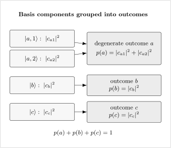
Distinct eigenvectors with the same eigenvalue belong to one outcome projector. Their squared component magnitudes add to the probability $p(a)$; nondegenerate outcomes require only one component.

Coarse-Grained Outcomes

A measurement may report a set $S$ of fine outcomes as one coarse result. The coarse projector is

$$P_S = \sum_{a\in S} P_a.$$

Because the fine projectors are orthogonal,

$$P_S^2 = P_S,$$

and

$$\begin{aligned} p(S) &= \operatorname{Tr}(\rho P_S)\\ &= \sum_{a\in S} \operatorname{Tr}(\rho P_a)\\ &= \sum_{a\in S}p(a). \end{aligned}$$

The probabilities add because the fine outcomes are mutually exclusive records of the declared projective measurement. This is different from coherent alternatives that lead to the same unresolved amplitude before a measurement.

Matrix Calculation

In an orthonormal computational basis, represent a pure state by a column $c$ and an outcome projector by a matrix $P_a$. Then

$$p(a) = c^\dagger P_a c.$$

The projected branch is the column $P_ac$, and

$$c^\dagger P_ac = (P_ac)^\dagger(P_ac)$$

because $P_a^\dagger P_a=P_a$.

For a nondegenerate measurement performed in the computational basis,

$$P_n = \operatorname{diag} \left( 0,\ldots,0,1,0,\ldots \right),$$

so the matrix formula selects

$$p(n) = \lvert c_n\rvert^2.$$

The same calculation works in any basis provided the state and projectors are represented consistently.

Mixed States

For a density operator,

$$p(a) = \operatorname{Tr}(\rho P_a).$$

In a measurement basis adapted to a degenerate eigenspace,

$$p(a) = \sum_{\alpha=1}^{d_a} \rho_{a\alpha,a\alpha}.$$

Only the diagonal entries in this measurement basis contribute directly to the displayed distribution. Off-diagonal entries are not thereby unphysical: they can affect probabilities for another measurement basis.

For an ensemble

$$\rho = \sum_k w_k \lvert\psi_k\rangle \langle\psi_k\rvert,$$

linearity of the trace gives

$$p(a) = \sum_k w_k \langle\psi_k\rvert P_a\lvert\psi_k\rangle.$$

The result depends only on $\rho$, not on a particular ensemble decomposition. The state theory is developed in Density Operators.

When the State Is Given in Another Basis

Suppose the state is given in an orthonormal basis $\{\lvert e_n\rangle\}$:

$$\lvert\psi\rangle = \sum_n c_n\lvert e_n\rangle.$$

For a nondegenerate measurement basis $\{\lvert a\rangle\}$, define the overlap matrix

$$S_{an} = \langle a\rvert e_n\rangle.$$

The measurement-basis amplitudes are

$$d_a = \langle a\rvert\psi\rangle = \sum_n S_{an}c_n,$$

and

$$p(a) = \lvert d_a\rvert^2.$$

For a degenerate outcome, compute all amplitudes $d_{a\alpha}$ inside the eigenspace and sum their squared moduli:

$$p(a) = \sum_\alpha \lvert d_{a\alpha}\rvert^2.$$

Probability in Different Bases owns the detailed translation workflow and its qubit examples.

Outcome Values Do Not Weight Probabilities

For

$$A = \sum_a aP_a,$$

the eigenvalue $a$ labels the reported outcome. It does not multiply the Born probability:

$$p(a) \neq a\, \operatorname{Tr}(\rho P_a).$$

Eigenvalues enter expectation values,

$$\langle A\rangle = \sum_a a\,p(a),$$

only after the outcome probabilities have been found. Confusing these two steps is a common source of negative or non-normalized “probabilities.”

Worked Example: Spin Measurement

Write a normalized spin-$1/2$ state in the $S_z$ basis:

$$\lvert\psi\rangle = \cos\frac{\theta}{2} \lvert+z\rangle + e^{i\phi} \sin\frac{\theta}{2} \lvert-z\rangle.$$

The spectral projectors are

$$P_\pm = \lvert\pm z\rangle \langle\pm z\rvert.$$

Therefore

$$\begin{aligned} p\left(+\frac{\hbar}{2}\right) &= \cos^2\frac{\theta}{2},\\ p\left(-\frac{\hbar}{2}\right) &= \sin^2\frac{\theta}{2}. \end{aligned}$$

The phase $\phi$ does not affect the $S_z$ distribution, but it can affect spin measurements along another axis.

Worked Example: Finite-Level Energy

For a Hamiltonian with discrete spectral decomposition

$$H = \sum_E E P_E,$$

an ideal energy measurement has probabilities

$$p(E) = \operatorname{Tr}(\rho P_E).$$

For a nondegenerate pure-state expansion

$$\lvert\psi\rangle = \sum_n c_n\lvert E_n\rangle,$$

this becomes

$$p(E_n) = \lvert c_n\rvert^2.$$

If several states share one energy $E$, their weights must be grouped through $P_E$. Degeneracy is common in systems with rotational or other symmetries; an energy readout need not resolve the additional quantum numbers.

Worked Example: A Degenerate Three-Level Observable

In the orthonormal basis $\{\lvert0\rangle,\lvert1\rangle,\lvert2\rangle\}$, define

$$A = 0 \left( \lvert0\rangle\langle0\rvert + \lvert1\rangle\langle1\rvert \right) + 2\lvert2\rangle\langle2\rvert.$$

The two outcome projectors are

$$\begin{aligned} P_0 &= \lvert0\rangle\langle0\rvert + \lvert1\rangle\langle1\rvert,\\ P_2 &= \lvert2\rangle\langle2\rvert. \end{aligned}$$

For

$$\lvert\psi\rangle = \frac{ \lvert0\rangle +i\lvert1\rangle +2\lvert2\rangle }{\sqrt6},$$

the probabilities are

$$\begin{aligned} p(0) &= \langle\psi\rvert P_0\lvert\psi\rangle = \frac13,\\ p(2) &= \langle\psi\rvert P_2\lvert\psi\rangle = \frac23. \end{aligned}$$

The outcome $0$ does not distinguish which vector within its two-dimensional eigenspace contributed.

Countably Infinite Outcomes

Let $\{\lvert n\rangle\}_{n=0}^\infty$ be an orthonormal basis and choose $0\leq q<1$. The state

$$\lvert\psi_q\rangle = \sqrt{1-q} \sum_{n=0}^{\infty} q^{n/2}\lvert n\rangle$$

is normalized because

$$(1-q) \sum_{n=0}^{\infty} q^n = 1.$$

A measurement in this basis gives the geometric distribution

$$p(n) = (1-q)q^n.$$

The probability of a tail event is

$$\begin{aligned} \Pr(n\geq N) &= \sum_{n=N}^{\infty} (1-q)q^n\\ &= q^N. \end{aligned}$$

For countably infinite spectra, normalization is a convergence statement. The amplitude sequence must lie in $\ell^2$, and probabilities must be summed with the appropriate limiting procedure.

Certain and Impossible Outcomes

For a pure state,

$$P_a\lvert\psi\rangle = \lvert\psi\rangle \quad \Longrightarrow \quad p(a)=1,$$

while

$$P_a\lvert\psi\rangle = 0 \quad \Longrightarrow \quad p(a)=0.$$

More generally, $0<p(a)<1$ when the state has nonzero components both inside and outside the outcome subspace.

For a density operator, certainty means that the support of $\rho$ lies within $\operatorname{ran}P_a$; impossibility means that the support is orthogonal to that subspace.

Truncating an Infinite Basis

Numerical calculations often retain only $\lvert0\rangle,\ldots,\lvert N\rangle$. The retained projector is

$$P_{\leq N} = \sum_{n=0}^{N} \lvert n\rangle\langle n\rvert.$$

For the geometric example,

$$\langle\psi_q\rvert P_{\leq N} \lvert\psi_q\rangle = 1-q^{N+1}.$$

If the truncated state is not renormalized, its listed probabilities sum to the retained weight rather than one. Renormalizing changes the question to a conditional distribution given $n\leq N$:

$$p_N(n) = \frac{ (1-q)q^n }{ 1-q^{N+1} }, \qquad 0\leq n\leq N.$$

The missing tail probability $q^{N+1}$ should be monitored as a truncation error, not silently discarded.

Projector and Probability Diagnostics

Before trusting a discrete calculation, verify the measurement data:

$$\begin{aligned} P_a^\dagger&=P_a, & P_a^2&=P_a,\\ P_aP_b&=0 \quad(a\neq b), & \sum_aP_a&=I. \end{aligned}$$

Then verify the output:

$$p(a)\in[0,1], \qquad \sum_ap(a)=1.$$

In numerical work, small deviations can arise from floating-point error. Large imaginary parts, negative probabilities, or substantial failure of normalization usually indicate inconsistent bases, nonprojective candidate matrices, or an incompletely represented state space.

Probability and State Update Are Different

The Born rule answers

$$\text{How likely is outcome }a?$$

It does not by itself answer

$$\text{What state follows after outcome }a?$$

For an ideal projective measurement, a common conditional update is

$$\rho \longmapsto \frac{ P_a\rho P_a }{ \operatorname{Tr}(\rho P_a) },$$

when $p(a)>0$. The probability formula is the same for other instruments that can produce different conditional states. The update theory belongs to Projective Measurement and State Update Rule.

A Reliable Calculation Workflow

1. List distinct outcomes. Group repeated eigenvalues into one outcome.
2. Construct the projectors. Use the full eigenspace for every degenerate outcome.
3. Check the PVM. Verify orthogonality and completeness.
4. Normalize the state. For countable expansions, check convergence as well as the formal sum.
5. Align representations. Express the state and projectors in the same basis.
6. Apply the rule. Use $\lvert\langle a\rvert\psi\rangle\rvert^2$ only for rank-one pure-state outcomes; otherwise use a projected norm or trace.
7. Coarse-grain after fine probabilities are defined. Sum mutually exclusive outcome probabilities or their projectors.
8. Audit the result. Check reality, nonnegativity, and unit total probability.
9. Treat update separately. Do not infer a conditional state from $p(a)$ alone.

Common Mistakes

• Squaring an amplitude rather than taking its squared modulus.
• Reading coefficients in the preparation basis as probabilities for a different measurement basis.
• Treating a repeated eigenvalue as several distinct outcomes when the apparatus reports only the eigenvalue.
• Using one eigenvector instead of the full projector for a degenerate outcome.
• Multiplying the probability by the numerical eigenvalue.
• Assuming coefficient phases never matter because they disappear in one particular basis measurement.
• Forgetting to verify that candidate projectors are orthogonal and complete.
• Applying pure-state formulas directly to a mixed state without choosing a valid ensemble-independent expression.
• Assuming a finite truncation remains normalized without checking the omitted tail.
• Confusing the outcome probability with the post-measurement state.

Canonical Boundaries and Cross-Links

• Born Rule owns the state–effect probability postulate, POVMs, spectral events, and foundational boundary.
• Probability Amplitudes owns coherent addition and amplitude composition.
• Probability in Different Bases owns systematic basis translation before probabilities are computed.
• Born Rule for Continuous Spectra owns densities, intervals, generalized eigenstates, and mixed spectra.
• Projectors and Spectral Decomposition own the operator construction of sharp outcomes.
• Density Operators owns mixed-state structure and ensemble nonuniqueness.

References

• M. Born, “Zur Quantenmechanik der Stoßvorgänge”, Zeitschrift für Physik 37, 863–867 (1926).
• P. A. M. Dirac, The Principles of Quantum Mechanics, 4th ed., Oxford University Press, 1958. Develops transformation amplitudes and projection measurements.
• B. C. Hall, Quantum Theory for Mathematicians, Springer, 2013. Gives a mathematically careful account of Hilbert-space states, spectral theory, and projective probability measures.
• A. Peres, Quantum Theory: Concepts and Methods, Kluwer, 1995. Emphasizes operational distinctions among preparations, projectors, and outcomes.
• J. J. Sakurai and J. Napolitano, Modern Quantum Mechanics, 3rd ed., Cambridge University Press, 2020. Treats spin, compatible observables, degeneracy, and measurement postulates.
• R. Shankar, Principles of Quantum Mechanics, 2nd ed., Springer, 1994. Gives detailed finite-dimensional and basis-based calculations.

Exercises

Exercise 1: Two-level amplitudes

Let

$$\lvert\psi\rangle = \frac{ 2\lvert0\rangle-i\lvert1\rangle }{\sqrt5}.$$

Find the probabilities for a measurement in the $\{\lvert0\rangle,\lvert1\rangle\}$ basis.

Solution

The basis amplitudes are $2/\sqrt5$ and $-i/\sqrt5$. Therefore

$$p(0) = \frac45, \qquad p(1) = \frac15.$$

The probabilities are nonnegative and sum to one.

Exercise 2: Measurement in another basis

For the state in Exercise 1, compute the probabilities for the basis

$$\lvert\pm\rangle = \frac{ \lvert0\rangle\pm\lvert1\rangle }{\sqrt2}.$$

Solution

The amplitudes are

$$\begin{aligned} \langle+\rvert\psi\rangle &= \frac{2-i}{\sqrt{10}},\\ \langle-\rvert\psi\rangle &= \frac{2+i}{\sqrt{10}}. \end{aligned}$$

Hence

$$p(+) = p(-) = \frac{4+1}{10} = \frac12.$$

The original coefficients could not be squared directly because this is a different measurement basis.

Exercise 3: Degenerate outcome

Let

$$P_a = \lvert0\rangle\langle0\rvert + \lvert1\rangle\langle1\rvert, \qquad P_b = \lvert2\rangle\langle2\rvert,$$

and

$$\lvert\chi\rangle = \frac{ \lvert0\rangle-\lvert1\rangle }{\sqrt2}.$$

Find $p(a)$ and $p(b)$.

Solution

The state lies entirely in $\operatorname{ran}P_a$:

$$P_a\lvert\chi\rangle = \lvert\chi\rangle, \qquad P_b\lvert\chi\rangle = 0.$$

Therefore

$$p(a)=1, \qquad p(b)=0.$$

The relative minus sign does not remove the state from the two-dimensional outcome subspace.

Exercise 4: Matrix projectors

In a three-dimensional basis, take

$$\begin{aligned} P_A &= \begin{pmatrix} 1&0&0\\ 0&0&0\\ 0&0&1 \end{pmatrix},\\[2mm] P_B &= \begin{pmatrix} 0&0&0\\ 0&1&0\\ 0&0&0 \end{pmatrix}. \end{aligned}$$

and

$$c = \frac1{\sqrt6} \begin{pmatrix} 1\\ i\\ 2 \end{pmatrix}.$$

Verify that the matrices form a PVM and compute the probabilities.

Solution

Both matrices are Hermitian and idempotent. They are orthogonal and complete:

$$P_AP_B=0, \qquad P_A+P_B=I.$$

The probabilities are

$$\begin{aligned} p(A) &= c^\dagger P_Ac = \frac{1+4}{6} = \frac56,\\ p(B) &= c^\dagger P_Bc = \frac16. \end{aligned}$$

Exercise 5: Coherence in a density matrix

Consider

$$\rho = \begin{pmatrix} \frac12&\gamma\\ \gamma^*&\frac12 \end{pmatrix}, \qquad \lvert\gamma\rvert\leq\frac12.$$

Find the outcome probabilities in the $z$ basis and in the $\{\lvert+\rangle,\lvert-\rangle\}$ basis.

Solution

The $z$-basis probabilities are the diagonal entries:

$$p(0)=p(1)=\frac12.$$

For the complementary basis,

$$\begin{aligned} p(+) &= \langle+\rvert\rho\lvert+\rangle = \frac12+\operatorname{Re}\gamma,\\ p(-) &= \langle-\rvert\rho\lvert-\rangle = \frac12-\operatorname{Re}\gamma. \end{aligned}$$

The off-diagonal coherence is invisible to the $z$ measurement but affects the complementary measurement.

Exercise 6: Countably infinite distribution

For $0\leq q<1$, let

$$\begin{aligned} p(n)&=(1-q)q^n,\\ n&=0,1,2,\ldots. \end{aligned}$$

verify normalization and find $\Pr(n\geq N)$.

Solution

The geometric series gives

$$\sum_{n=0}^{\infty} p(n) = (1-q) \frac1{1-q} = 1.$$

The tail is

$$\begin{aligned} \Pr(n\geq N) &= (1-q) \sum_{n=N}^{\infty} q^n\\ &= (1-q) \frac{q^N}{1-q} = q^N. \end{aligned}$$

Exercise 7: Coarse-graining

A four-outcome PVM gives

$$\begin{aligned} p_0&=\frac1{10}, & p_1&=\frac2{10},\\ p_2&=\frac3{10}, & p_3&=\frac4{10}. \end{aligned}$$

Outcomes $2$ and $3$ are reported together as $S$. Find $P_S$ and $p(S)$.

Solution

The coarse projector and probability are

$$P_S = P_2+P_3$$

and

$$p(S) = p_2+p_3 = \frac7{10}.$$

Orthogonality of $P_2$ and $P_3$ ensures that $P_S$ is again a projector.

Exercise 8: Finite truncation

For the geometric distribution in Exercise 6, retain only $n=0,\ldots,N$. Find the retained probability and the normalized conditional distribution within the truncation.

Solution

The retained probability is

$$\begin{aligned} p(n\leq N) &= (1-q) \sum_{n=0}^{N} q^n\\ &= 1-q^{N+1}. \end{aligned}$$

Conditioning on the retained subspace gives

$$p_N(n) = \frac{ (1-q)q^n }{ 1-q^{N+1} }, \qquad 0\leq n\leq N.$$

The omitted tail has probability $q^{N+1}$.