Expectation Values

The expectation value of an observable is the first moment of its Born-rule probability distribution. Operationally, it is the average approached by many measurements on independently and identically prepared systems, provided the relevant expectation exists.

For a normalized pure state $|\psi\rangle$ and a self-adjoint observable $A$, the familiar operator formula is

$$\langle A\rangle_\psi = \langle\psi|A|\psi\rangle.$$

For a density operator $\rho$, the corresponding formula is

$$\langle A\rangle_\rho = \operatorname{Tr}(\rho A).$$

For an unbounded observable, this notation presupposes a finite absolute first spectral moment, $\operatorname{Tr}(\rho |A|)<\infty$; the trace is then understood through the spectral integral. Without that condition, the mean need not exist.

These compact expressions are consequences of the Born rule. They do not say that a single measurement will return $\langle A\rangle$, nor that the system possesses this number before measurement. This page owns the quantum measurement meaning and operator formulation of expectation values. Generic probability facts are developed at Expectation Values in Probability, while detailed mixed-state trace calculations belong to Trace Rule for Expectation Values.

Required background. The Born Rule supplies the outcome distribution whose first moment is taken.

Helpful background. Spectral Decomposition supplies the observable’s spectral events; Expectation Values in Probability reviews discrete and continuous means.

Expected measurement outcome

Let $\mu_\rho^A$ be the Born probability measure of $A$ in the state $\rho$:

$$\mu_\rho^A(\Delta) = \operatorname{Tr}\!\left[ \rho P^A(\Delta) \right].$$

The expectation value is

$$\langle A\rangle_\rho = \int_{\mathbb R}\lambda\,d\mu_\rho^A(\lambda),$$

when the integral is well defined. This definition makes the statistical content explicit: each possible outcome $\lambda$ is weighted by its Born probability.

The notation $\langle A\rangle$ suppresses the state. That shorthand is safe only when the state is clear from context. The same observable can have very different expectations in different states.

Repeated measurements and sample means

Prepare $N$ independent systems in the same state $\rho$, measure $A$ once on each, and denote the outcomes by $a_1,\ldots,a_N$. The empirical mean is

$$\overline A_N = \frac{1}{N}\sum_{j=1}^{N}a_j.$$

If the outcome distribution has a finite absolute first moment, the law of large numbers gives

$$\overline A_N \longrightarrow \langle A\rangle_\rho$$

with probability one as $N\to\infty$. Thus expectation values are testable ensemble predictions, not merely algebraic decorations on operators.

For finite $N$, the sample mean fluctuates. If the variance is finite and the trials are independent, its standard deviation is

$$\Delta\overline A_N = \frac{\Delta A}{\sqrt N}.$$

This $N^{-1/2}$ statistical uncertainty is distinct from calibration errors, state-preparation drift, and detector systematics. The intrinsic spread $\Delta A$ is treated canonically at Variance and Standard Deviation.

Expectation is not the most likely outcome

The mean, mode, and median answer different questions:

• The expectation value is a probability-weighted average.
• A mode is an outcome with maximal probability or density.
• A median divides the probability into two halves.

They need not coincide. The expectation need not even be a possible individual outcome.

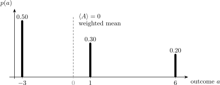
For outcomes $-3$, $1$, and $6$ with probabilities $0.50$, $0.30$, and $0.20$, the expectation is $0$. It is neither an allowed outcome nor the most likely outcome, which is $-3$.

For this example,

$$\begin{aligned} \langle A\rangle &= (-3)(0.50)+(1)(0.30)\\ &\qquad{} +(6)(0.20)=0. \end{aligned}$$

The value zero summarizes the distribution’s first moment. It does not predict that any trial will produce zero.

Discrete outcomes

Suppose $A$ has a finite or countable spectral decomposition

$$A = \sum_a aP_a,$$

where $P_a$ projects onto the full eigenspace with eigenvalue $a$. The Born probability is

$$p_\rho(a) = \operatorname{Tr}(\rho P_a),$$

and the expectation is

$$\langle A\rangle_\rho = \sum_a a\,p_\rho(a).$$

For a pure state,

$$p_\psi(a) = \langle\psi|P_a|\psi\rangle,$$

so

$$\langle A\rangle_\psi = \sum_a a\, \langle\psi|P_a|\psi\rangle.$$

Degeneracy requires no extra probability rule: $P_a$ already includes every orthogonal state in the eigenspace. If a basis $|a,r\rangle$ resolves a degeneracy label $r$, then

$$p_\psi(a) = \sum_r |\langle a,r|\psi\rangle|^2.$$

The canonical probability calculation is at Born Rule for Discrete Spectra.

Continuous outcomes

If the state-dependent spectral measure admits a density $p_A(\lambda)$ with respect to $d\lambda$, then

$$\langle A\rangle_\rho = \int_{-\infty}^{\infty} \lambda p_A(\lambda)\,d\lambda.$$

For one-dimensional position in a pure state,

$$\langle X\rangle_\psi = \int_{-\infty}^{\infty} x|\psi(x)|^2\,dx.$$

The density has inverse-outcome units, so the integrand times $d\lambda$ has the units of the observable. The full treatment of densities, atoms, and coordinate changes is at Born Rule for Continuous Spectra.

Mixed spectra

An observable may have atomic weights $w_n$ at eigenvalues $a_n$ and an absolutely continuous density $p_{\mathrm{ac}}(\lambda)$. Its expectation is

$$\langle A\rangle_\rho = \sum_n a_n w_n + \int_{\mathbb R} \lambda p_{\mathrm{ac}}(\lambda)\,d\lambda.$$

One must include both parts. Integrating only the continuum omits occupied bound-state components; summing only eigenvalues omits scattering outcomes. The measure expression

$$\langle A\rangle_\rho = \int_{\mathbb R}\lambda\,d\mu_\rho^A(\lambda)$$

handles discrete, continuous, singular, and mixed spectral measures in one line.

Deriving the operator formula

The spectral theorem represents a self-adjoint operator as

$$A = \int_{\mathbb R}\lambda\,P^A(d\lambda).$$

For a pure state, taking the quadratic form gives

$$\begin{aligned} \langle\psi|A|\psi\rangle &= \int_{\mathbb R}\lambda\, \langle\psi|P^A(d\lambda)|\psi\rangle\\ &= \int_{\mathbb R}\lambda\, d\mu_\psi^A(\lambda). \end{aligned}$$

This is exactly the probability-theory expectation. The operator expression and the weighted-outcome expression are not separate postulates; they are two representations of the same Born-rule statistic.

The practical spectral construction is developed at Spectral Decomposition.

Why the expectation is real

Because $A$ is self-adjoint,

$$\begin{aligned} \langle\psi|A|\psi\rangle^* &= \langle A\psi|\psi\rangle\\ &= \langle\psi|A\psi\rangle. \end{aligned}$$

Hence

$$\langle A\rangle_\psi\in\mathbb R.$$

In a finite-dimensional numerical calculation, a significant imaginary part usually signals that the matrix is not Hermitian, the state or inner-product convention was implemented incorrectly, or rounding errors are poorly controlled. For differential operators, bad boundary conditions or a domain mismatch can produce the same symptom.

Density operators and the trace rule

For a density operator $\rho$ with $\operatorname{Tr}(\rho|A|)<\infty$, the expectation is

$$\langle A\rangle_\rho = \operatorname{Tr}(\rho A).$$

In any orthonormal basis $\{|n\rangle\}$,

$$\operatorname{Tr}(\rho A) = \sum_n\langle n|\rho A|n\rangle.$$

If

$$\rho = \sum_j q_j|\psi_j\rangle\langle\psi_j|,$$

then

$$\langle A\rangle_\rho = \sum_j q_j \langle\psi_j|A|\psi_j\rangle.$$

The result depends only on $\rho$, not on which ensemble decomposition is used to represent it. The cyclicity, basis independence, local-observable formulas, and unbounded-operator cautions of the trace expression are developed at Trace Rule for Expectation Values.

Linearity

Expectation is linear in the observable. For real $\alpha$ and $\beta$,

$$\langle\alpha A+\beta B\rangle_\rho = \alpha\langle A\rangle_\rho + \beta\langle B\rangle_\rho,$$

whenever the required expectations and operator domains are well defined. The observables $A$ and $B$ need not commute. This is a statement about ensemble means, not about the existence of a joint sharp measurement.

Linearity does not imply factorization:

$$\langle AB\rangle_\rho \ne \langle A\rangle_\rho\langle B\rangle_\rho$$

in general. Correlations, operator ordering, and noncommutativity matter for products.

Functions of an observable and moments

The functional calculus gives

$$f(A) = \int_{\mathbb R}f(\lambda)\,P^A(d\lambda).$$

Therefore

$$\langle f(A)\rangle_\rho = \int_{\mathbb R}f(\lambda)\, d\mu_\rho^A(\lambda),$$

provided the expectation exists. Taking $f(\lambda)=\lambda^n$ produces the moments

$$\langle A^n\rangle_\rho = \int_{\mathbb R}\lambda^n\, d\mu_\rho^A(\lambda).$$

In particular,

$$(\Delta A)^2 = \langle A^2\rangle_\rho - \langle A\rangle_\rho^2.$$

Knowing only $\langle A\rangle$ does not determine the distribution. Many different Born distributions share the same first moment.

Eigenstates and certainty

If

$$A|a\rangle=a|a\rangle,$$

then

$$\langle A\rangle_a=a, \qquad \langle A^2\rangle_a=a^2, \qquad \Delta A=0.$$

Every measurement of $A$ in that state returns $a$ in the ideal projective model.

The converse requires the zero-spread condition. Merely finding $\langle A\rangle=a$ does not prove that the state is an eigenstate, even if $a$ happens to be an eigenvalue. Contributions above and below $a$ can average to the same number.

Bounds and the convex hull of outcomes

If a bounded observable satisfies

$$mI\le A\le MI,$$

then every state obeys

$$m\le\langle A\rangle_\rho\le M.$$

For a finite spectrum, the expectation is a convex combination of eigenvalues and lies in their convex hull. For a two-outcome observable with eigenvalues $a_-$ and $a_+$,

$$\langle A\rangle = a_-p_-+a_+p_+, \qquad p_-+p_+=1,$$

so the mean lies between the two outcomes. It need not equal either one.

These bounds are valuable sanity checks. A computed spin expectation outside the operator’s spectral interval is necessarily wrong.

Basis and matrix formulas

Choose an orthonormal basis and represent the normalized state by a column vector $\mathbf c$. Then

$$\langle A\rangle_\psi = \mathbf c^\dagger A\mathbf c.$$

Under a unitary basis change,

$$\mathbf c' = U^\dagger\mathbf c, \qquad A' = U^\dagger A U.$$

The scalar is unchanged:

$$\mathbf c'^{\dagger}A'\mathbf c' = \mathbf c^\dagger A\mathbf c.$$

An expectation value is representation independent even though the state components and operator matrix change.

Example: a qubit observable

Write a qubit state and Hermitian observable as

$$\rho = \frac12\bigl(I+\mathbf r\cdot\boldsymbol\sigma\bigr), \qquad A = a_0I+\mathbf a\cdot\boldsymbol\sigma.$$

Using $\operatorname{Tr}(\sigma_i)=0$ and $\operatorname{Tr}(\sigma_i\sigma_j)=2\delta_{ij}$ gives

$$\langle A\rangle_\rho = a_0+\mathbf r\cdot\mathbf a.$$

For $A=\sigma_z$ and $|\psi\rangle=\alpha|0\rangle+\beta|1\rangle$,

$$\langle\sigma_z\rangle_{\psi} = |\alpha|^2-|\beta|^2.$$

The outcomes are $+1$ and $-1$. Any expectation in $[-1,1]$ is possible, even though values strictly between the endpoints are not single-shot outcomes.

Example: energy in a superposition

Let $H|E_n\rangle=E_n|E_n\rangle$ and

$$|\psi\rangle = \sum_n c_n|E_n\rangle.$$

Then

$$\langle H\rangle_{\psi} = \sum_n |c_n|^2E_n.$$

Relative phases among the $c_n$ do not affect the energy probabilities because $H$ is diagonal in this basis. For an observable $B$ that is not diagonal in the energy basis,

$$\langle B\rangle_{\psi} = \sum_{m,n}c_m^*c_n B_{mn},$$

and off-diagonal terms can make relative phases observable.

Wavefunction representations

In a position representation, a pure-state expectation is formally

$$\langle A\rangle_{\psi} = \int_{-\infty}^{\infty} \psi^*(x)(A\psi)(x)\,dx.$$

For position,

$$\langle X\rangle_{\psi} = \int_{-\infty}^{\infty} x|\psi(x)|^2\,dx.$$

For momentum in the standard coordinate representation,

$$\langle P\rangle_{\psi} = \int_{-\infty}^{\infty} \psi^*(x) \left(-i\hbar\frac{d}{dx}\right) \psi(x)\,dx.$$

The second expression is real only when the state lies in the relevant self-adjoint domain and the boundary terms are controlled. The page Expectation Values in Wave Mechanics owns coordinate-space calculations, integration by parts, radial measures, and numerical quadrature.

Existence and unbounded observables

Normalization of the state does not guarantee that every expectation is finite. The measure-theoretic expectation exists as a finite number when

$$\int_{\mathbb R}|\lambda|\, d\mu_\rho^A(\lambda) <\infty.$$

For a pure state and unbounded $A$, the operator expression $\langle\psi|A|\psi\rangle$ is certainly defined when $|\psi\rangle$ lies in the operator domain $D(A)$. The expectation can also be handled through the associated quadratic form under the appropriate weaker integrability condition. Domain claims should therefore accompany formal differential-operator manipulations.

Higher moments require stronger conditions. A state can have finite $\langle|A|\rangle$ but infinite $\langle A^2\rangle$, so its mean exists while its variance does not.

Symmetry does not rescue a divergent mean

Consider the normalized even density

$$p(x) = \frac{1}{2(1+|x|)^2}.$$

The positive and negative tails appear to cancel in a symmetric principal value, but

$$\int_{-\infty}^{\infty}|x|p(x)\,dx =\infty.$$

Therefore the ordinary expectation of $X$ is undefined, not zero. Assigning a value by symmetric cancellation confuses a Cauchy principal value with a Lebesgue expectation. This distinction matters whenever outcome distributions have heavy tails.

Generalized measurements

For a discrete POVM with numerical outcomes $y$ and effects $E_y$,

$$p(y) = \operatorname{Tr}(\rho E_y), \qquad \sum_y E_y=I.$$

Its expectation is

$$\begin{aligned} \mathbb E[Y] &= \sum_y y\,\operatorname{Tr}(\rho E_y)\\ &= \operatorname{Tr}(\rho M_1), \end{aligned}$$

where

$$M_1 = \sum_y yE_y$$

is the POVM’s first-moment operator. Different POVMs can share the same $M_1$ while having different full distributions and higher moments. Measuring the sharp observable $M_1$ is therefore not generally equivalent to performing the original POVM.

See POVMs: First Encounter for generalized measurement probabilities and effects.

Time dependence and classical-looking motion

In the Schrödinger picture, both the state and an explicitly time-dependent observable may contribute to the evolution of an expectation. Under the usual domain assumptions,

$$\frac{d}{dt}\langle A\rangle = \frac{i}{\hbar}\langle[H,A]\rangle + \left\langle\frac{\partial A}{\partial t}\right\rangle.$$

This equation does not turn an ensemble mean into a classical trajectory, but for position and momentum it leads to equations resembling classical mechanics under suitable conditions. The interpretation and approximation limits are at Ehrenfest Theorem Overview.

Common mistakes

Predicting a single result

An expectation is an ensemble statistic. A single projective measurement returns a spectral outcome, not generally the mean.

Confusing mean and mode

The most probable outcome can differ sharply from the mean. For a continuous law, the mode concerns density height, whereas the expectation depends on the entire weighted tail structure.

Forgetting the state

$\langle A\rangle$ is incomplete notation unless the state is understood. The observable alone does not determine its expectation.

Omitting degeneracy or continuum sectors

Probabilities must be summed over every unresolved degeneracy label and over all atomic and continuous spectral components.

Using unnormalized states

For a nonzero but unnormalized vector $|\phi\rangle$, the normalized expression is

$$\langle A\rangle_{\phi} = \frac{\langle\phi|A|\phi\rangle} {\langle\phi|\phi\rangle}.$$

The denominator cannot be silently omitted.

Ignoring domains and convergence

Square-integrability of a wavefunction does not ensure a finite expectation for every unbounded observable. Check operator domains, boundary conditions, and absolute moment convergence.

Factoring products

In general $\langle AB\rangle\ne\langle A\rangle\langle B\rangle$. Factorization requires additional statistical or state structure.

Inferring the distribution from one moment

A mean alone does not determine probabilities, variance, skewness, tails, or whether the spectrum is discrete or continuous.

Summary

The Born rule defines the state-dependent spectral measure $\mu_\rho^A$. Its first moment is the expectation value:

$$\langle A\rangle_\rho = \int_{\mathbb R}\lambda\, d\mu_\rho^A(\lambda).$$

Equivalent operator formulas are

$$\langle A\rangle_\psi = \langle\psi|A|\psi\rangle, \qquad \langle A\rangle_\rho = \operatorname{Tr}(\rho A),$$

under the appropriate domain and convergence assumptions. The expectation is real, linear in the observable, basis independent, and constrained by the spectral range for bounded observables. It is estimated by repeated measurements, need not be an allowed single-shot outcome, and need not exist for a normalized state with sufficiently heavy spectral tails.

References

• P. Busch, P. J. Lahti, J.-P. Pellonpää, and K. Ylinen, Quantum Measurement, Springer, 2016, Chapters 3–5.
• P. A. M. Dirac, The Principles of Quantum Mechanics, 4th ed., Oxford University Press, 1958, Chapters II–III.
• B. C. Hall, Quantum Theory for Mathematicians, Springer, 2013, Chapters 7–10.
• M. Reed and B. Simon, Methods of Modern Mathematical Physics, Vol. I: Functional Analysis, revised and enlarged ed., Academic Press, 1980, Sections VII.1–VII.3 and VIII.3.
• J. J. Sakurai and J. Napolitano, Modern Quantum Mechanics, 3rd ed., Cambridge University Press, 2020, Chapters 1–2.
• R. Shankar, Principles of Quantum Mechanics, 2nd ed., Springer, 1994, Chapters 1 and 4.
• J. von Neumann, Mathematical Foundations of Quantum Mechanics, Princeton University Press, 1955, Chapters II–III.

Exercises

1. A three-outcome observable

An observable has outcomes $-2$, $1$, and $4$ with probabilities $1/4$, $1/2$, and $1/4$. Compute its expectation. Is the expectation an allowed outcome?

Solution

The expectation is

$$\begin{aligned} \langle A\rangle &= (-2)\frac14+(1)\frac12+(4)\frac14\\ &=1. \end{aligned}$$

Here the expectation happens to equal the allowed outcome $1$. That coincidence does not imply that every measurement returns $1$; the other outcomes still have total probability $1/2$.

2. Mean versus most likely result

A two-outcome observable returns $0$ with probability $0.9$ and $20$ with probability $0.1$. Find the mean and the mode. Explain why neither alone fully describes the experiment.

Solution

The mean is

$$\mathbb E[A] = (0)(0.9)+(20)(0.1) =2,$$

while the unique mode is $0$. The mean $2$ is not a possible outcome, and the mode omits the rare but large result $20$. The full probability distribution is needed to predict all frequencies.

3. Matrix expectation and basis change

Let

$$A = \begin{pmatrix} 2 & i\\ -i & -1 \end{pmatrix}, \qquad |\psi\rangle = \frac{1}{\sqrt5} \begin{pmatrix} 1\\ 2 \end{pmatrix}.$$

Compute $\langle A\rangle_\psi$. Why must the answer be real despite the complex matrix entries?

Solution

First,

$$A|\psi\rangle = \frac{1}{\sqrt5} \begin{pmatrix} 2+2i\\ -i-2 \end{pmatrix}.$$

Therefore

$$\begin{aligned} \langle A\rangle_\psi &= \frac15 \begin{pmatrix}1&2\end{pmatrix} \begin{pmatrix}2+2i\\-i-2\end{pmatrix}\\ &= -\frac25. \end{aligned}$$

The imaginary terms cancel because $A=A^\dagger$. A simultaneous unitary change of the state components and operator matrix would leave this scalar unchanged.

4. Phase-sensitive qubit expectation

For

$$|\psi\rangle = \cos\frac{\theta}{2}|0\rangle + e^{i\varphi}\sin\frac{\theta}{2}|1\rangle,$$

compute $\langle\sigma_x\rangle$. Which relative phase gives the largest value at fixed $\theta$?

Solution

Because

$$\sigma_x = |0\rangle\langle1|+|1\rangle\langle0|,$$

the expectation is the sum of the two cross terms:

$$\begin{aligned} \langle\sigma_x\rangle &= 2\cos\frac{\theta}{2} \sin\frac{\theta}{2}\cos\varphi\\ &= \sin\theta\cos\varphi. \end{aligned}$$

At fixed $\theta$ with $\sin\theta\ge0$, this is largest for $\varphi=0$ modulo $2\pi$. The example shows that relative phase can affect an expectation when the observable is not diagonal in the preparation basis.

5. Expectation from symmetry

Let $p(x)$ be a normalized, even position density with a finite absolute first moment. Show that $\langle X\rangle=0$. Why is the integrability assumption essential?

Solution

Since $p(-x)=p(x)$, the function $xp(x)$ is odd. Absolute integrability permits the positive and negative halves to be combined legitimately:

$$\begin{aligned} \langle X\rangle &= \int_{-\infty}^{\infty}xp(x)\,dx\\ &= \int_0^\infty x[p(x)-p(-x)]\,dx =0. \end{aligned}$$

Without $\int |x|p(x)dx<\infty$, the two half-line integrals may diverge. A symmetric principal value can then vanish even though the ordinary expectation does not exist.

6. A normalized state with no position mean

Verify that

$$p(x)=\frac{1}{2(1+|x|)^2}$$

is normalized, and show that $\mathbb E[|X|]$ diverges.

Solution

Evenness gives

$$\int_{-\infty}^{\infty}p(x)\,dx = \int_0^\infty\frac{dx}{(1+x)^2} =1.$$

For the absolute first moment,

$$\mathbb E[|X|] = \int_0^\infty\frac{x}{(1+x)^2}\,dx.$$

The integrand behaves as $1/x$ for large $x$, so the integral diverges logarithmically. The probability law is normalized, but its position expectation is undefined.

7. Energy expectation and relative phase

Let

$$|\psi\rangle = \frac{1}{\sqrt2} \left(|E_1\rangle+e^{i\phi}|E_2\rangle\right),$$

where $H|E_j\rangle=E_j|E_j\rangle$ and $E_1\ne E_2$. Find $\langle H\rangle$. Does it depend on $\phi$?

Solution

Orthogonality and diagonal action of $H$ give

$$\langle H\rangle = \frac{E_1+E_2}{2}.$$

It is independent of $\phi$ because the energy probabilities are both $1/2$. The relative phase can still affect expectations of observables with nonzero off-diagonal matrix elements between $|E_1\rangle$ and $|E_2\rangle$.

8. Statistical precision

An observable has standard deviation $\Delta A=3$ in a fixed state. Assuming independent preparations and negligible systematics, how many measurements are needed to make the standard deviation of the sample mean at most $0.03$?

Solution

The sample-mean standard deviation is

$$\Delta\overline A_N = \frac{3}{\sqrt N}.$$

Requiring this to be at most $0.03$ gives

$$\frac{3}{\sqrt N}\le0.03, \qquad \sqrt N\ge100,$$

so $N\ge10^4$. This quantifies statistical precision only; systematic errors do not generally decrease as $N^{-1/2}$.