Time-Dependent Perturbation Theory and Transitions

Time-dependent perturbation theory asks how a weak, explicitly time-varying interaction changes quantum amplitudes. It is the standard entry point for driven transitions, absorption and stimulated emission, finite-duration pulses, decay into continua, and the transition-rate limit summarized by Fermi’s golden rule.

The method begins with

$$H(t)=H_0+\lambda V(t),$$

but its logic differs from static perturbation theory. The main outputs are not corrected stationary energies. They are amplitudes that accumulate in time, probabilities that begin at quadratic order in the coupling, and, only under additional assumptions, rates that become approximately constant over an intermediate time window.

This chapter owns that approximation hierarchy. Exact picture transformations and formal time-ordered evolution retain their canonical homes in Interaction Picture and Dyson Expansion as Formal Evolution. Coherent two-level dynamics belong to Rabi Oscillations: First Encounter, while this chapter explains when their weak-drive limit may be used perturbatively.

The Central Setup

Assume that the reference Hamiltonian is solved:

$$H_0\lvert n\rangle = E_n\lvert n\rangle.$$

Prepare the system at time $t_0$ in a known state, often one eigenstate $\lvert i\rangle$ of $H_0$. The perturbation $\lambda V(t)$ acts during a specified time interval. The basic question is:

What is the amplitude to find the system in a chosen final state $\lvert f\rangle$ at time $t$?

The bookkeeping parameter $\lambda$ identifies perturbative order and is set to its physical value at the end. A useful split requires more than a formally small coefficient. The evolution generated by $H_0$ should be tractable, the matrix elements of $V(t)$ should be identifiable, and the accumulated transition probability should remain in the regime claimed by the truncation.

A transition is relative to a basis

A transition means a change in the probabilities associated with a specified set of states or measurement outcomes. Usually those states are eigenstates of $H_0$, because their phase evolution is known and their energy differences define the resonant frequencies. In that basis,

$$\omega_{fi} = \frac{E_f-E_i}{\hbar}$$

is the Bohr angular frequency for the pair $i\to f$.

The word “transition” should not be read as a microscopic movie of an instantaneous jump. During coherent evolution the state can be a superposition of several reference eigenstates. A projective energy measurement at the final time samples the corresponding probabilities.

The basis statement matters. A perturbation diagonal in one basis changes phases without changing populations in that basis, while those phases may alter interference in another measurement basis.

Why the Interaction Picture Is the Workbench

Let

$$U_0(t,t_0) = e^{-iH_0(t-t_0)/\hbar}.$$

Define the interaction-picture state and perturbation by

$$\lvert\psi_I(t)\rangle = U_0^\dagger(t,t_0) \lvert\psi_S(t)\rangle,$$ $$V_I(t) = U_0^\dagger(t,t_0) V(t) U_0(t,t_0).$$

The exact Schrödinger equation becomes

$$i\hbar \frac{d}{dt}\lvert\psi_I(t)\rangle = \lambda V_I(t) \lvert\psi_I(t)\rangle.$$

The known $H_0$ motion has been removed from the state, leaving only interaction-driven evolution. Integrating once gives

$$\begin{aligned} \lvert\psi_I(t)\rangle ={}& \lvert\psi_I(t_0)\rangle \\ &- \frac{i\lambda}{\hbar} \int_{t_0}^{t}dt_1\, V_I(t_1) \lvert\psi_I(t_1)\rangle. \end{aligned}$$

Iterating this integral equation produces the Dyson series. Before truncation, that series is a formal representation of exact evolution. After truncation in $\lambda$, it becomes time-dependent perturbation theory. Keeping those two statements separate prevents a common confusion: time ordering itself is not an approximation.

Amplitudes Before Probabilities

Expand the interaction-picture state in the $H_0$ basis:

$$\lvert\psi_I(t)\rangle = \sum_n c_n(t)\lvert n\rangle.$$

If the initial state is $\lvert i\rangle$, then

$$c_n(t_0)=\delta_{ni}.$$

The exact coefficient equations are

$$i\hbar\dot c_f(t) = \lambda \sum_n \langle f\rvert V_I(t)\lvert n\rangle c_n(t).$$

At first order, replace the coefficients on the right by their initial values. For $f\ne i$,

$$c_f^{(1)}(t) = -\frac{i}{\hbar} \int_{t_0}^{t}dt'\, e^{i\omega_{fi}(t'-t_0)} V_{fi}(t'),$$

where

$$V_{fi}(t)=\langle f\rvert V(t)\lvert i\rangle.$$

The full coefficient is

$$c_f(t) = \lambda c_f^{(1)}(t) +O(\lambda^2), \qquad f\ne i.$$

Consequently, the leading transition probability is

$$P_{i\to f}(t) = \lambda^2 \lvert c_f^{(1)}(t)\rvert^2 +O(\lambda^3).$$

The conventional phrase “first-order transition probability” means the probability obtained from the first-order amplitude. The probability itself starts at second order in the coupling.

For the initial channel $f=i$, the first-order term commonly contains a phase. Probability conservation couples the survival probability to second-order amplitudes and to the sum of transition probabilities. One should not mix a first-order survival amplitude with a second-order transition probability and expect exact normalization.

The detailed derivation, square-pulse examples, and normalization checks belong to First-Order Transition Probability.

Transitions as Spectral Matching

The first-order integral combines two oscillations:

1. the intrinsic phase $e^{i\omega_{fi}t}$ set by the energy gap;
2. the frequency content of the applied perturbation.

Suppose one component of the matrix element has the form

$$V_{fi}(t) = W_{fi}f(t)e^{-i\omega t},$$

where $f(t)$ is an envelope. Then

$$c_f^{(1)}(t) = -\frac{iW_{fi}}{\hbar} \int_{t_0}^{t}dt'\, f(t')e^{i\Delta_{fi}t'},$$

up to an irrelevant phase from the choice of time origin, with detuning

$$\Delta_{fi}=\omega_{fi}-\omega.$$

The amplitude samples the finite-time Fourier transform of the pulse envelope at the detuning. Resonance is therefore phase accumulation with little cancellation, not a singularity in the exact finite-time problem.

Square pulse

For $f(t)=1$ on $0\le t\le T$,

$$\begin{aligned} I_T(\Delta) &= \int_0^Tdt\,e^{i\Delta t} \\ &= T e^{i\Delta T/2} \operatorname{sinc}\!\left(\frac{\Delta T}{2}\right), \end{aligned}$$

where $\operatorname{sinc}x=\sin x/x$. The leading probability is

$$P_{i\to f}^{(1)}(T) = \frac{\lambda^2\lvert W_{fi}\rvert^2}{\hbar^2} T^2 \operatorname{sinc}^2\!\left(\frac{\Delta_{fi}T}{2}\right).$$

At exact resonance, the first-order amplitude grows as $T$ and the probability as $T^2$. This growth signals eventual breakdown of the undepleted first-order approximation; it does not predict an indefinitely growing physical probability.

Away from resonance, positive and negative phase contributions cancel. Increasing the pulse duration narrows the range of detunings that add coherently, with characteristic width

$$\delta\omega\sim\frac{1}{T}.$$

This finite-time spectral resolution is often loosely described using an energy–time uncertainty relation. No time operator is required: the width follows directly from Fourier analysis of a finite-duration drive.

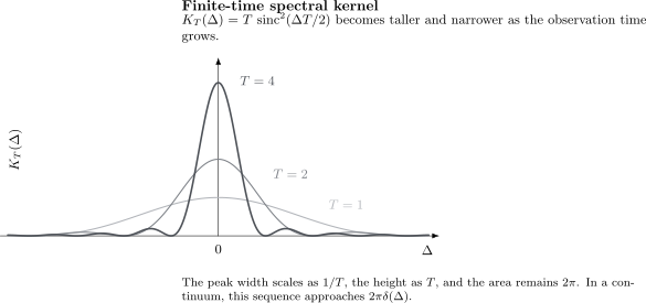
The normalized finite-time kernel $K_T(\Delta)=\lvert I_T(\Delta)\rvert^2/T$ has fixed area. Longer observation times increase its peak and narrow its frequency width. This is the distributional step that converts a continuum transition probability into an approximately constant rate.

For a general envelope, the line shape is its Fourier power spectrum. Abrupt switching produces broad sinc sidelobes; smooth switching suppresses high-frequency content. The physical switching protocol is therefore part of the model, not a disposable mathematical detail.

Discrete States and Continua

The same first-order amplitude leads to different physical descriptions depending on the final spectrum.

Discrete final state

For one isolated final level, $P_{i\to f}(T)$ remains a coherent finite-time probability. Under a monochromatic drive it has resonance structure and, beyond weak first order, usually crosses over to bounded coherent oscillation. A constant transition rate is not the generic description of a closed two-level system.

Continuum of final states

For a dense spectrum, a sum over final states may become

$$\sum_f \longrightarrow \int dE\,\rho(E),$$

where $\rho(E)$ is a density of states defined with a stated normalization. The finite-time kernel obeys the distributional limit

$$\lim_{T\to\infty} \frac{\lvert I_T(\Delta)\rvert^2}{T} = 2\pi\delta(\Delta).$$

If the matrix element and density of states vary slowly across the kernel width, integration over the continuum gives

$$\Gamma_{i\to f} = \frac{2\pi}{\hbar} \lambda^2 \lvert W_{fi}\rvert^2 \rho(E_f),$$

evaluated at the energy selected by the drive. This is the simplest form of Fermi’s Golden Rule.

The order of operations matters. At finite $T$, the kernel is an ordinary function and the probability begins quadratically in time. The linear-in-$T$ behavior appears only after summing over a sufficiently dense set of final states and entering a time window in which the kernel resolves the smooth continuum without resolving its microscopic level spacing.

Three Time Regimes

There is no universal “long-time limit.” Several scales compete.

Regime	Typical condition	Behavior	Appropriate description
Very short time	$T$ shorter than inverse spectral widths	$P_{i\to f}\propto T^2$	Finite-time amplitude; no constant rate
Golden-rule window	Correlations have decayed, but depletion and recurrences are small	Total probability grows approximately as $\Gamma T$	Continuum rate
Late time	$\Gamma T$ is not small, levels are spectrally resolved, or recurrences occur	Depletion, coherent oscillation, linewidth, or recurrence	Resummation, open-system, or exact dynamics

A common schematic hierarchy is

$$\tau_{\mathrm{corr}} \ll T \ll \min\!\left(\Gamma^{-1},\tau_{\mathrm{rec}}\right).$$

Here $\tau_{\mathrm{corr}}$ measures the memory or spectral-correlation time of the final-state manifold, and $\tau_{\mathrm{rec}}$ is a recurrence time associated with its finite level spacing. The left inequality permits a rate description; the right inequalities keep depletion and discreteness from invalidating it.

The short-time quadratic law is also the starting point for the quantum Zeno effect, but repeated measurements and open-system dynamics are separate canonical topics. This chapter uses the short-time law only as a perturbative consistency check.

Matrix Elements Carry the Physics

Frequency matching alone does not guarantee a transition. The perturbation matrix element

$$V_{fi}(t)=\langle f\rvert V(t)\lvert i\rangle$$

contains geometry, symmetry, polarization, and coupling strength. If a symmetry forces $V_{fi}=0$, the first-order transition is forbidden even at exact resonance.

The division of labor is:

• Selection Rules derives symmetry constraints on operator matrix elements;
• Selection Rules in Transition Rates inserts those zeros and weights into perturbative probabilities and rates;
• Harmonic Perturbations separates absorption-like, emission-like, rotating, and counter-rotating terms.

Selection rules are exact only under the symmetry assumptions used to derive them. Weak symmetry breaking can make a forbidden transition weakly allowed, often at a higher perturbative order or through state mixing.

Spectroscopy and Scattering Connections

Spectroscopy

In a semiclassical light–matter model, an electric field couples through an operator such as

$$V(t)=-\mathbf d\mathbin{\cdot}\mathbf E(t).$$

The transition amplitude combines the pulse spectrum with the dipole matrix element. Resonant frequencies reveal level differences; polarization and angular dependence probe tensor structure; and line strengths probe squared matrix elements. Real spectra also contain broadening from finite lifetimes, collisions, inhomogeneity, and instrumental response, none of which is supplied automatically by first-order perturbation theory.

The experimental role of spectra is introduced in Spectroscopy, while angular-momentum structure belongs to the symmetry volume.

Scattering

Scattering theory also compares prepared incoming states with possible outgoing states. Its transition operator, asymptotic limits, state normalization, and flux factors require a dedicated framework, but the perturbative logic is related: amplitudes are primary, squared amplitudes enter probabilities or cross sections, continuum normalization supplies densities of final states, and time-translation symmetry enforces energy conservation.

The canonical scattering construction begins at Scattering Amplitude and Cross Sections. The bridge to relativistic notation is QFT Bridge: S-Matrix.

Method Map

Question	Start here
How is the solvable motion separated from the perturbation?	Interaction Picture
How is that split turned into coefficient equations and phase estimates?	Interaction Picture for Perturbation Theory
Where do time ordering and perturbative terms come from?	Dyson Expansion as Formal Evolution
How do ordered interaction insertions generate transition paths?	Dyson Expansion for Transition Amplitudes
What is the leading transition amplitude and probability?	First-Order Transition Probability
How does a sinusoidal drive create resonance?	Harmonic Perturbations
What sets the resonance condition, linewidth, and breakdown time?	Resonant Driving
How does the exact Rabi result reduce to first order?	Rabi Formula in the Weak-Drive Limit
When does a probability become a rate?	Fermi’s Golden Rule
How do transition amplitudes become a susceptibility and absorbed power?	Linear Response Preview
How do dipole matrix elements become absorption and emission rates?	Transition Rates in Light–Matter Interaction
How do symmetry zeros affect rates?	Selection Rules in Transition Rates
When does coherent population transfer replace first order?	Rabi Oscillations: First Encounter
What happens during a sweep through an avoided crossing?	Landau–Zener Transition
How does the continuum final-state measure enter a rate?	Density of States in Transition Rates
What happens when the Hamiltonian changes too quickly for the state to follow?	Sudden Approximation
How are slow evolution, leakage, and runtime estimated?	Adiabatic Approximation as a Method

Validity Ledger

A mature transition calculation records the following.

Item	Question to answer
Hamiltonian split	Why is $H_0$ solvable and why is $\lambda V(t)$ the smaller interaction?
Initial preparation	What state or density operator is prepared at $t_0$?
Switching protocol	When and how is the perturbation applied and removed?
Target basis	Which final states define the claimed transitions?
Spectral scale	What detuning, pulse bandwidth, level spacing, or continuum width matters?
Matrix element	Which symmetry and normalization conventions determine $V_{fi}$?
Truncation	Which amplitude orders are retained, and what probability accuracy follows?
Observation window	Is the result short-time, coherent finite-time, golden-rule, or asymptotic?

For one target channel, a useful diagnostic is

$$\epsilon_{fi}(t) = \frac{\lvert\lambda\rvert}{\hbar} \left\lvert \int_{t_0}^{t}dt'\, e^{i\omega_{fi}t'}V_{fi}(t') \right\rvert.$$

First order requires $\epsilon_{fi}\ll1$ for every channel whose depletion is neglected. More globally, define

$$P_{\mathrm{loss}}(t) = \sum_{f\ne i}P_{i\to f}(t).$$

The undepleted initial-state approximation requires

$$P_{\mathrm{loss}}(t)\ll1.$$

This condition can fail at resonance or after long times even when the instantaneous perturbation is weak. Small coupling and long evolution do not commute automatically.

An operator-norm estimate,

$$\epsilon_{\mathrm{norm}}(t) = \frac{\lvert\lambda\rvert}{\hbar} \int_{t_0}^{t}dt'\, \lVert V_I(t')\rVert,$$

is a conservative sufficient diagnostic in bounded finite-dimensional problems. It may be too crude to capture oscillatory cancellation, and it is not automatically meaningful for unbounded operators. Channel-specific phases and physical spectral scales usually give the sharper estimate.

Common Mistakes

• Calling the leading probability first order in the coupling. The first-order amplitude produces an $O(\lambda^2)$ probability for a previously empty channel.
• Dropping the interaction-picture phase. The factor $e^{i\omega_{fi}t}$ is what compares the drive spectrum with the energy gap.
• Replacing the finite-time kernel by a delta function too early. At finite time, the resonance has nonzero width and the very-short-time probability is quadratic.
• Using a rate for an isolated two-level system. Coherent discrete dynamics generally require a bounded oscillatory solution rather than indefinite linear growth.
• Ignoring the switching envelope. Pulse shape controls bandwidth and sidelobes and can create transitions absent in an ideal infinite sinusoid.
• Treating resonance as sufficient. A vanishing matrix element forbids the first-order transition even when the frequencies match.
• Forgetting continuum normalization. The dimensions of matrix elements and densities of states depend on whether states are normalized to one, to volume, or to delta functions.
• Extending first order beyond depletion. Secular growth is a breakdown warning, not a prediction of probability greater than one.
• Equating time ordering with perturbation. The time-ordered evolution operator is formal and exact; truncating its Dyson expansion is the approximation.
• Using “energy conservation” for an arbitrary drive. A time-dependent field can supply or remove energy; the relevant condition includes its frequency content.

Exercises

Identify the transition basis

A two-level Hamiltonian has $H_0=(\hbar\omega_0/2)\sigma_z$ and perturbation $V(t)=v(t)\sigma_z$. Does the perturbation cause transitions between the $H_0$ energy eigenstates? Can it still affect a measurement in the $\sigma_x$ basis?

Solution

Because $V(t)$ is diagonal in the $\sigma_z$ basis,

$$\langle -z\rvert V(t)\lvert +z\rangle=0.$$

It therefore causes no transitions between the two $H_0$ energy eigenstates. It does change their relative phase:

$$\phi_+(t)-\phi_-(t) = -\frac{2}{\hbar} \int_{t_0}^{t}v(t')\,dt'.$$

A state with both $\sigma_z$ components can consequently acquire different $\sigma_x$ measurement probabilities. Population transfer is basis dependent, while the full unitary evolution is not.

Derive the first-order amplitude

Starting from

$$i\hbar\dot c_f(t) = \lambda\sum_n(V_I)_{fn}(t)c_n(t),$$

with $c_n(t_0)=\delta_{ni}$, derive the first-order amplitude for $f\ne i$.

Solution

At zeroth order, only $c_i^{(0)}=1$ is nonzero. The first-order equation is therefore

$$i\hbar\dot c_f^{(1)}(t) = (V_I)_{fi}(t).$$

Integrating from $t_0$ and using $c_f^{(1)}(t_0)=0$ gives

$$c_f^{(1)}(t) = -\frac{i}{\hbar} \int_{t_0}^{t}dt'\,(V_I)_{fi}(t').$$

For $H_0$ eigenstates,

$$(V_I)_{fi}(t') = e^{i\omega_{fi}(t'-t_0)}V_{fi}(t'),$$

which yields the stated amplitude formula. The physical coefficient includes the prefactor $\lambda$.

Check the square-pulse limits

For a square harmonic pulse, show that

$$P_{i\to f}^{(1)}(T) = \frac{\lambda^2\lvert W_{fi}\rvert^2}{\hbar^2} T^2 \operatorname{sinc}^2\!\left(\frac{\Delta T}{2}\right).$$

Find its resonant value and its universal short-time behavior at fixed detuning.

Solution

The amplitude contains

$$\begin{aligned} I_T(\Delta) &= \int_0^Tdt\,e^{i\Delta t} \\ &= T e^{i\Delta T/2} \operatorname{sinc}\!\left(\frac{\Delta T}{2}\right). \end{aligned}$$

Taking its squared magnitude gives the stated result. On resonance, $\Delta=0$ and $\operatorname{sinc}(0)=1$, so

$$P_{i\to f}^{(1)}(T) = \frac{\lambda^2\lvert W_{fi}\rvert^2}{\hbar^2}T^2.$$

At fixed detuning and sufficiently short time, $\lvert\Delta T\rvert\ll1$, so the same quadratic law holds to leading order. The system has not yet evolved long enough to resolve the detuning.

Recover the golden-rule factor

Let continuum states be labeled by energy with density $\rho(E)$. Use

$$\frac{\lvert I_T(\Delta)\rvert^2}{T} \longrightarrow 2\pi\delta(\Delta)$$

to derive the rate for absorption from a drive of frequency $\omega$, where $\Delta=(E-E_i)/\hbar-\omega$.

Solution

The total leading probability is

$$P(T) = \frac{\lambda^2}{\hbar^2} \int dE\, \rho(E)\lvert W_{Ei}\rvert^2 \lvert I_T(\Delta)\rvert^2.$$

Divide by $T$ and take the continuum long-time limit:

$$\begin{aligned} \Gamma ={}& \frac{2\pi\lambda^2}{\hbar^2} \int dE\, \rho(E)\lvert W_{Ei}\rvert^2 \\ &\times \delta\!\left( \frac{E-E_i}{\hbar}-\omega \right). \end{aligned}$$

Since

$$\delta\!\left( \frac{E-E_i}{\hbar}-\omega \right) = \hbar\delta(E-E_i-\hbar\omega),$$

the result is

$$\Gamma = \frac{2\pi}{\hbar} \lambda^2 \rho(E_i+\hbar\omega) \lvert W_{E_i+\hbar\omega,i}\rvert^2.$$

This step also shows why the density-of-states convention and the Jacobian must be tracked together.

Audit probability orders

Suppose $c_f=\lambda a_f+\lambda^2b_f+O(\lambda^3)$ for $f\ne i$. Through which order is $P_{i\to f}$ known if only $a_f$ is calculated? What additional amplitude information is needed for the next correction?

Solution

Squaring gives

$$\begin{aligned} P_{i\to f} ={}& \lambda^2\lvert a_f\rvert^2 \\ &+2\lambda^3 \operatorname{Re}(a_f^*b_f) +O(\lambda^4). \end{aligned}$$

Knowing only the first-order amplitude $a_f$ determines the leading $O(\lambda^2)$ probability. The $O(\lambda^3)$ probability requires the second-order amplitude $b_f$. If symmetries make the interference term vanish, the next nonzero correction may occur later, but that must be demonstrated rather than assumed.

Decide whether a rate is justified

A system couples to a dense band with correlation time $2\,\mathrm{fs}$, golden-rule lifetime $4\,\mathrm{ns}$, and finite-size recurrence time $50\,\mathrm{ps}$. Identify a reasonable qualitative time window for a constant-rate description.

Solution

The rate picture requires times long compared with the correlation time but short compared with both depletion and recurrence:

$$2\,\mathrm{fs} \ll T \ll \min(4\,\mathrm{ns},50\,\mathrm{ps}).$$

Thus a useful window is schematically

$$2\,\mathrm{fs}\ll T\ll50\,\mathrm{ps}.$$

The inequalities are parametric, not sharp boundaries. Close to either endpoint, finite-memory or recurrence corrections must be checked.

Cross-Links

• Approximation Volume Overview
• Small Parameters and Error Estimates
• Interaction Picture
• Interaction Picture for Perturbation Theory
• Dyson Expansion as Formal Evolution
• Dyson Expansion for Transition Amplitudes
• First-Order Transition Probability
• Harmonic Perturbations
• Resonant Driving
• Rabi Formula in the Weak-Drive Limit
• Fermi’s Golden Rule
• Density of States in Transition Rates
• Selection Rules in Transition Rates
• Sudden Approximation
• Adiabatic Approximation as a Method
• Landau–Zener Transition
• Linear Response Preview
• Transition Rates in Light–Matter Interaction
• Rabi Oscillations: First Encounter
• Green Functions and Density of States
• Scattering Amplitude

References

• P. A. M. Dirac, The Principles of Quantum Mechanics, 4th ed., Oxford University Press, 1958.
• C. Cohen-Tannoudji, B. Diu, and F. Laloë, Quantum Mechanics, Vol. 2, Wiley, 1977.
• J. J. Sakurai and J. Napolitano, Modern Quantum Mechanics, 3rd ed., Cambridge University Press, 2020.
• A. Messiah, Quantum Mechanics, Vol. 2, Dover, 1999.
• R. Shankar, Principles of Quantum Mechanics, 2nd ed., Springer, 1994.
• C. J. Joachain, Quantum Collision Theory, 3rd ed., North-Holland, 1983.
• B. Zwiebach, Quantum Physics III, MIT OpenCourseWare 8.06, 2018.