Resonant Driving

Resonant driving occurs when a time-dependent perturbation has frequency content close enough to a quantum transition frequency that amplitudes generated at different times add coherently. Resonance is therefore a dynamical regime, not a literal divergence. Its location, width, and eventual saturation depend on the drive envelope, observation time, coupling strength, neighboring levels, and environmental broadening.

This page owns that regime analysis. Harmonic Perturbations owns the general first-order calculation for sinusoidal drives. Rabi Oscillations: First Encounter owns the bounded coherent dynamics of an isolated driven two-level system, and Rabi Formula in the Weak-Drive Limit owns the asymptotic match to transition theory. The Rotating-Wave Approximation owns the approximation that discards rapidly rotating terms.

Rabi Oscillations owns the AMO experimental continuation: coupling and intensity conventions, pulse-area calibration, measured traces, chevrons, readout, and departures from the isolated square-pulse model.

Resonance as Coherent Accumulation

Let the reference Hamiltonian have stationary states

$$H_0lvert n\rangle = E_nlvert n\rangle,$$

and define the Bohr angular frequency

$$\omega_{fi} = \frac{E_f-E_i}{\hbar}.$$

Consider a drive with carrier frequency $\omega$ and real envelope $f(t)$,

$$V(t) = f(t) \left( W e^{-i\omega t} + W^\dagger e^{i\omega t} \right).$$

For an upward transition with $\omega_{fi}\gt0$, the nearly stationary contribution to the first-order amplitude is

$$\begin{aligned} c_{f,\mathrm{rot}}^{(1)}(T) &= -\frac{i}{\hbar} W_{fi} \int_0^T dt\, f(t)e^{i\Delta t}, \\ \Delta &\equiv \omega_{fi}-\omega, \qquad W_{fi}=\langle f\rvert W\lvert i\rangle. \end{aligned}$$

The quantity $\Delta$ is the detuning. Introduce the finite-duration Fourier amplitude

$$F_T(\Delta) \equiv \int_0^T dt\,f(t)e^{i\Delta t}.$$

Then

$$c_{f,\mathrm{rot}}^{(1)}(T) = -\frac{i}{\hbar}W_{fi}F_T(\Delta).$$

This compact equation contains the basic resonance mechanism:

• $W_{fi}$ decides whether the transition is coupled at all;
• $F_T(\Delta)$ measures how much drive spectrum lies at the transition frequency;
• the phase of $F_T$ matters in coherent interference experiments;
• $\lvert F_T\rvert^2$ gives the first-order spectral line shape.

The counter-rotating term carries the much larger mismatch $\omega_{fi}+\omega$ for a positive-frequency near-resonant drive. Neglecting it is not part of the definition of resonance; it is an additional rotating-wave or averaging approximation whose validity must be checked.

The Resonance Condition

The shorthand statement

$$\hbar\omega \simeq E_f-E_i$$

means more than equality of two numbers. For a pulse of finite duration, useful resonance requires

$$\lvert\Delta\rvert \lesssim \delta\omega_{\mathrm{pulse}},$$

where $\delta\omega_{\mathrm{pulse}}$ is the spectral width of the envelope. It also requires

$$W_{fi}\ne0.$$

A frequency match cannot overcome an exact selection-rule zero. Conversely, a nonzero matrix element does not guarantee a large transition if the drive spectrum has negligible weight at $\omega_{fi}$.

For a nearly monochromatic pulse of duration $T$, the Fourier width is of order

$$\delta\omega_{\mathrm{pulse}} \sim \frac{1}{T}.$$

The numerical coefficient and the presence of sidelobes depend on the pulse shape. Saying only that a drive is “on resonance” is incomplete unless its envelope, duration, and frequency convention are specified.

Rectangular Pulse and Finite-Time Linewidth

Take a constant envelope switched on for $0\le t\le T$:

$$f(t)=1.$$

The Fourier amplitude is

$$\begin{aligned} F_T(\Delta) &= \int_0^Tdt\,e^{i\Delta t} \\ &= e^{i\Delta T/2} T\, \operatorname{sinc} \left( \frac{\Delta T}{2} \right), \end{aligned}$$

where

$$\operatorname{sinc}u \equiv \frac{\sin u}{u}, \qquad \operatorname{sinc}0=1.$$

The leading transition probability is therefore

$$P_{i\to f}^{(1)}(T) = \frac{\lvert W_{fi}\rvert^2T^2}{\hbar^2} \operatorname{sinc}^2 \left( \frac{\Delta T}{2} \right).$$

Define a positive coupling angular frequency by

$$\Omega \equiv \frac{2\lvert W_{fi}\rvert}{\hbar}.$$

With this convention,

$$P_{i\to f}^{(1)}(T) = \frac{\Omega^2T^2}{4} \operatorname{sinc}^2 \left( \frac{\Delta T}{2} \right).$$

At exact resonance,

$$P_{i\to f}^{(1)}(T) \longrightarrow \frac{\Omega^2T^2}{4}.$$

The apparent resonance denominator has disappeared. The correct $\Delta\to0$ limit is finite at fixed time and grows quadratically because the amplitude accumulates linearly.

First zeros

The nearest zeros satisfy

$$\frac{\Delta T}{2} = \pm\pi,$$

so they occur at

$$\Delta_{\mathrm{zero}} = \pm\frac{2\pi}{T}.$$

The zero-to-zero angular-frequency width of the central lobe is therefore

$$\delta\omega_{\mathrm{zero}} = \frac{4\pi}{T}.$$

Full width at half maximum

Let $u_{1/2}$ be the positive root of

$$\operatorname{sinc}^2u_{1/2} = \frac{1}{2}.$$

Numerically,

$$u_{1/2} \simeq 1.391557.$$

The full width at half maximum is

$$\begin{aligned} \delta\omega_{\mathrm{FWHM}} &= \frac{4u_{1/2}}{T} \\ &\simeq \frac{5.566}{T}. \end{aligned}$$

In ordinary frequency $\nu=\omega/(2\pi)$,

$$\delta\nu_{\mathrm{FWHM}} \simeq \frac{0.886}{T}.$$

These coefficients belong specifically to the squared sinc profile of a rectangular pulse. They are not universal linewidth constants.

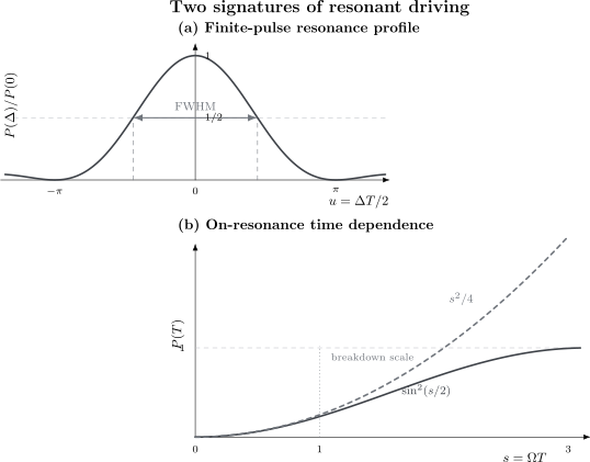
Left: a rectangular pulse gives the normalized profile $\operatorname{sinc}^2(\Delta T/2)$, with first zeros at $\Delta T/2=\pm\pi$ and half-maximum points at approximately $\pm1.39$. Right: on resonance, first-order theory agrees with $\sin^2(\Omega T/2)$ only while $\Omega T$ is small; the polynomial truncation is not bounded at long times.

Abrupt switching creates the sidelobes. They are a property of the rectangular time window, not extra energy levels. Smoother envelopes generally reduce sidelobes at the cost of a different central-lobe width.

Detuning and Phase Cancellation

The integrand in the rotating contribution is

$$e^{i\Delta t}.$$

At $\Delta=0$, every time slice contributes with the same phase. If $\Delta\ne0$, the phase advances, and contributions from later parts of the pulse partially cancel earlier ones. The phase changes by order one after a time

$$t_\phi \sim \frac{1}{\lvert\Delta\rvert}.$$

This gives a useful physical form of the resonance criterion:

$$T \lesssim t_\phi \quad\Longleftrightarrow\quad \lvert\Delta\rvert T \lesssim 1.$$

For a rectangular pulse, the probability is even in detuning,

$$P^{(1)}(\Delta) = P^{(1)}(-\Delta),$$

but the complex amplitude is not simply identical at opposite detunings because it includes the phase $e^{i\Delta T/2}$. Ramsey interferometry, composite pulses, and coherent control can therefore be sensitive to the sign of detuning even when a single-pulse population measurement is not.

Pulse Shape Is Part of the Physics

For a general weak pulse, the transition profile is

$$P_{i\to f}^{(1)} \propto \lvert F_T(\Delta)\rvert^2.$$

Thus line shape is Fourier analysis of the actual envelope. As a clean comparison, take a Gaussian amplitude envelope extending effectively over all time,

$$f(t) = \exp\left[ -\frac{(t-t_c)^2}{2\tau^2} \right].$$

Its transform is

$$F(\Delta) = \sqrt{2\pi}\,\tau e^{i\Delta t_c} \exp\left[ -\frac{\Delta^2\tau^2}{2} \right].$$

The probability profile is Gaussian,

$$\lvert F(\Delta)\rvert^2 = 2\pi\tau^2 e^{-\Delta^2\tau^2},$$

with angular-frequency full width at half maximum

$$\delta\omega_{\mathrm{FWHM}} = \frac{2\sqrt{\ln2}}{\tau}.$$

The parameter $\tau$ here is the standard deviation of the amplitude envelope as written. Different communities quote intensity widths, root-mean-square widths, or $1/e$ widths; converting conventions is essential before comparing numerical linewidths.

Finite-time resolution is sometimes summarized as an energy–time uncertainty relation. No time operator is needed for this result. The width follows directly from the Fourier transform of the preparation and observation protocol; see Energy–Time Uncertainty for the distinctions among several energy–time statements.

Why First Order Breaks Down on Resonance

Weak coupling does not by itself guarantee a uniformly valid approximation for arbitrarily long resonant driving. With the convention above, the first-order on-resonance amplitude has magnitude

$$\lvert c_f^{(1)}(T)\rvert = \frac{\Omega T}{2}.$$

The corresponding perturbative requirement is

$$\Omega T \ll 1.$$

More generally, a useful finite-time expansion parameter for the selected transition is

$$\epsilon_T(\Delta) \equiv \frac{\Omega T}{2} \left\lvert \operatorname{sinc} \left( \frac{\Delta T}{2} \right) \right\rvert.$$

First-order transition theory requires

$$\epsilon_T(\Delta) \ll 1,$$

together with small amplitudes into every other appreciably coupled state.

On exact resonance, successive Dyson terms also accumulate coherently. The expansion is nonuniform in time: terms small at fixed $T$ cease to be small when $T$ scales as $1/\Omega$. A prediction such as

$$P_{i\to f}^{(1)}(T)\gt1$$

is not a physical probability. It is a diagnostic that the truncation has been used beyond its domain.

This is the same kind of secular behavior encountered elsewhere in perturbation theory. The cure is to resum the resonant dynamics, solve the relevant few-level problem, or use an effective Hamiltonian that treats the near-degenerate resonant subspace nonperturbatively.

Exact Two-Level Bridge

For an isolated two-level system under a monochromatic drive, suppose a rotating-frame transformation and the rotating-wave approximation lead to

$$H_{\mathrm{eff}} = \frac{\hbar}{2} \left( \Delta\sigma_z + \Omega\sigma_x \right).$$

This effective Hamiltonian is not the exact description of every resonantly driven system. Under its assumptions, however, the transition probability from one bare level to the other is

$$P_{i\to f}(T) = \frac{\Omega^2}{\Omega_R^2} \sin^2\left( \frac{\Omega_RT}{2} \right),$$

where

$$\Omega_R = \sqrt{\Omega^2+\Delta^2}$$

is the generalized Rabi angular frequency.

At exact resonance,

$$P_{i\to f}(T) = \sin^2\left( \frac{\Omega T}{2} \right).$$

Its short-time expansion is

$$P_{i\to f}(T) = \frac{\Omega^2T^2}{4} + O\!\left((\Omega T)^4\right),$$

which reproduces first-order transition theory while remaining bounded when the perturbative polynomial fails.

For fixed nonzero detuning, fixed $\Delta T$, and weak coupling,

$$\begin{aligned} P_{i\to f}(T) &= \frac{\Omega^2}{\Delta^2} \sin^2\left( \frac{\Delta T}{2} \right) \\ &\quad +O\!\left( \frac{\Omega^4}{\Delta^4} \right). \end{aligned}$$

Using $\operatorname{sinc}x=\sin x/x$, the leading term is exactly

$$\frac{\Omega^2T^2}{4} \operatorname{sinc}^2 \left( \frac{\Delta T}{2} \right).$$

The exact and perturbative descriptions therefore overlap, but their small parameters must be stated. Near resonance the relevant condition is $\Omega T\ll1$; far off resonance, the transition remains small when $\Omega/\lvert\Delta\rvert\ll1$. Over extremely long times, higher-order frequency shifts can still accumulate an order-one phase error even while the population transfer stays small.

The complete two-level interpretation, including Bloch-sphere geometry, is developed in Rabi Oscillations: First Encounter.

Pulse Area on Exact Resonance

The resonant breakdown can also be expressed through pulse area. In a two-level rotating-wave model with fixed drive phase, let the coupling vary as $\Omega(t)$. On exact resonance, the effective Hamiltonians at different times are proportional to the same Pauli matrix and therefore commute. Define

$$\mathcal A \equiv \int_{t_0}^{t_1}dt\,\Omega(t).$$

The exact transition probability is then

$$P_{i\to f} = \sin^2\left( \frac{\mathcal A}{2} \right).$$

First order gives only

$$P_{i\to f}^{(1)} = \frac{\mathcal A^2}{4}.$$

The perturbative regime is $\lvert\mathcal A\rvert\ll1$. A pulse with $\mathcal A=\pi$ is a population-inverting $\pi$ pulse in the ideal model, far outside first-order transition theory even if its instantaneous coupling is weak compared with the carrier frequency.

The pulse-area formula requires exact resonance and a fixed coupling axis. Detuning, phase modulation, chirp, counter-rotating corrections, additional levels, and dissipation generally make time ordering nontrivial.

Distinct Sources of Linewidth

The word “linewidth” can refer to different physical mechanisms. They should not be merged into a single $1/T$ slogan.

Origin	Characteristic scale	Typical profile	What it means
Finite interrogation or pulse duration	$1/T$	Envelope-dependent; sinc-squared for a rectangular pulse	Fourier-limited resolution of a coherent protocol
Lifetime and homogeneous dephasing	$1/T_1$ and $1/T_2$	Often Lorentzian in a Markovian steady-state model	Loss of population or phase coherence
Strong continuous drive	set by $\Omega$ together with relaxation rates	Power-broadened steady-state response	Saturation and driven dressed-state dynamics
Static or slowly varying disorder	spread of transition frequencies	Often Gaussian or a convolution	Inhomogeneous ensemble broadening
Motion	Doppler or recoil scales	Geometry- and distribution-dependent	Frequency shifts sampled across a velocity distribution

Only the first row is derived by the finite rectangular-pulse calculation. Homogeneous broadening and saturation require an open-system model such as the Optical Bloch Equations. Inhomogeneous broadening requires averaging over the relevant ensemble distribution.

An isolated, perfectly coherent two-level system under continuous drive does not settle into an irreversible transition rate. It undergoes Rabi oscillations. A constant rate emerges only after additional coarse graining, a continuum of final states, decoherence, stochasticity, or a specified measurement protocol. The continuum limit is treated in Fermi’s Golden Rule.

Resonance Centers Can Shift

The bare condition $\omega=\omega_{fi}$ is a starting point. The observed peak may move because of

• off-resonant coupling to other levels, producing AC Stark shifts;
• counter-rotating terms, producing a Bloch–Siegert shift;
• static fields and interactions that alter the level spacing;
• Doppler, recoil, collisional, or medium-dependent effects;
• calibration offsets in the drive and measurement chain.

These shifts are often second order in a weak coupling but become important precisely because modern spectroscopy can resolve frequencies much more accurately than the raw linewidth. A measured peak center should therefore be compared with the resonance condition of the full effective model, not automatically identified with the unperturbed gap.

Multilevel and Degenerate Systems

A two-level approximation is justified only when the selected pair is spectrally and dynamically isolated. A useful scale estimate is

$$B_{\mathrm{eff}} \sim \max\left\{ \frac{1}{T}, \lvert\Omega\rvert, \Gamma_2 \right\},$$

where $\Gamma_2$ denotes a representative coherence-decay rate when an open-system description is present. For every unwanted state $\lvert n\rangle$, one wants either a symmetry-forbidden matrix element or a detuning satisfying roughly

$$B_{\mathrm{eff}} \ll \lvert\omega_{ni}-\omega\rvert.$$

If several levels lie inside the effective bandwidth, the drive addresses a resonant manifold rather than one isolated transition. One must retain and diagonalize that coupled subspace. Dark states, bright states, interference among pathways, and Autler–Townes structure can then appear.

The leading order also matters. A one-photon transition uses the condition $\omega\simeq\omega_{fi}$ in first order. A multiphoton resonance may instead satisfy

$$m\omega \simeq \omega_{fi},$$

for an integer $m\gt1$, but its amplitude arises at higher order and involves intermediate-state denominators. Dyson Expansion for Transition Amplitudes provides the appropriate pathway bookkeeping.

Spectroscopic Interpretation

In weak-drive spectroscopy, scanning $\omega$ and recording a transition signal probes

$$\lvert W_{fi}\rvert^2 \lvert F_T(\omega_{fi}-\omega)\rvert^2,$$

modified by state preparation, detection efficiency, broadening, and shifts. The peak location estimates a transition frequency only after those effects are modeled. The peak area and height are not interchangeable: changing pulse duration can narrow the line while changing its height, even when the underlying matrix element is fixed.

The historical experimental logic is developed in Spectroscopy and Magnetic Resonance. The CW, pulsed, relaxation, and detector forward models are organized in Magnetic Resonance Overview.

A Reliable Workflow

1. Specify the reference spectrum. Record the states, gaps, degeneracies, and conventions for angular versus ordinary frequency.
2. Write the actual drive. Include its operator, polarization, carrier phase, envelope, switching, and duration.
3. Compute matrix elements. Apply selection rules before discussing resonance enhancement.
4. List every relevant detuning. Include the rotating, counter-rotating, neighboring-level, and possible multiphoton mismatches.
5. Fourier analyze the envelope. Use $F_T(\Delta)$ rather than inserting an exact delta function at finite time.
6. Name the linewidth mechanism. Distinguish Fourier width, homogeneous width, inhomogeneous width, and drive-induced broadening.
7. Check the accumulated coupling. Near resonance, test $\Omega T$ or the pulse area, not only the instantaneous ratio $\Omega/\omega$.
8. Escalate the model when needed. Use exact few-level dynamics, a rotating-frame effective Hamiltonian, Floquet theory, or an open-system equation according to the failed assumption.
9. Report the observable. State whether the calculation predicts a complex amplitude, a population after a pulse, a steady-state signal, or a transition rate.

Common Mistakes

• Calling the resonance denominator infinite. At finite time the integral has a smooth $\operatorname{sinc}$ limit; the divergent-looking expression came from an algebraic form used before taking $\Delta\to0$.
• Equating weak drive with valid first order forever. Resonant amplitudes accumulate, so $\Omega T$ can become order one even when $\Omega/\omega_{fi}$ is tiny.
• Treating $1/T$ as an intrinsic lifetime width. A finite pulse produces Fourier width even in a perfectly closed system.
• Using a delta function for one discrete final state. The long-time delta distribution becomes useful after integration over a smooth continuum, not as a literal finite-time probability for an isolated level.
• Ignoring the drive envelope. Hard and smooth switching have different sidelobes and linewidth coefficients.
• Forgetting matrix elements. Resonance enhances an allowed pathway; it does not erase symmetry constraints.
• Conflating the Rabi and rotating-wave approximations. Rabi oscillations are dynamics within a model; the rotating-wave approximation is one possible step used to obtain that model.
• Quoting a linewidth without a convention. Half width, full width, angular frequency, ordinary frequency, amplitude width, and intensity width differ by numerical factors.

Exercises

Rectangular-pulse widths

For

$$R(\Delta) = \operatorname{sinc}^2 \left( \frac{\Delta T}{2} \right),$$

find the first zeros and the full width at half maximum. You may use the numerical root $u_{1/2}=1.391557$ of $\operatorname{sinc}^2u=1/2$.

Solution

The first zeros occur when

$$\frac{\Delta T}{2} = \pm\pi,$$

so

$$\Delta = \pm\frac{2\pi}{T}.$$

The zero-to-zero width is $4\pi/T$. At half maximum,

$$\left\lvert \frac{\Delta T}{2} \right\rvert = u_{1/2}.$$

The two half-maximum detunings are $\Delta=\pm2u_{1/2}/T$, giving

$$\delta\omega_{\mathrm{FWHM}} = \frac{4u_{1/2}}{T} \simeq \frac{5.566}{T}.$$

Dividing by $2\pi$ gives $\delta\nu_{\mathrm{FWHM}}\simeq0.886/T$.

Secular growth and its cure

On resonance, compare the first-order prediction

$$P^{(1)}(T) = \frac{\Omega^2T^2}{4}$$

with the exact two-level result $P(T)=\sin^2(\Omega T/2)$. Through what order in $\Omega T$ do they agree, and at what time scale must first order fail?

Solution

Using

$$\sin^2x = x^2-\frac{x^4}{3}+O(x^6),$$

with $x=\Omega T/2$ gives

$$P(T) = \frac{\Omega^2T^2}{4} - \frac{\Omega^4T^4}{48} + O\!\left((\Omega T)^6\right).$$

The probabilities agree through order $(\Omega T)^2$. The relative correction becomes order one when $\Omega T\sim1$, so the resonant perturbative time scale is

$$T_{\mathrm{break}} \sim \frac{1}{\Omega}.$$

The exact result remains between zero and one; the polynomial truncation does not.

Off-resonant bound

For a rectangular pulse, show that when $\Delta\ne0$ the leading probability obeys

$$P_{i\to f}^{(1)}(T) \le \frac{\Omega^2}{\Delta^2}.$$

What time-independent small parameter does this suggest far from resonance?

Solution

Rewrite the probability as

$$P_{i\to f}^{(1)}(T) = \frac{\Omega^2}{\Delta^2} \sin^2\left( \frac{\Delta T}{2} \right).$$

Since $0\le\sin^2x\le1$,

$$P_{i\to f}^{(1)}(T) \le \frac{\Omega^2}{\Delta^2}.$$

Far from resonance, $\Omega/\lvert\Delta\rvert\ll1$ keeps the transition small even for observation times much longer than $1/\Omega$. This contrasts with exact resonance, where the relevant parameter is $\Omega T$.

Gaussian transform limit

For

$$f(t) = \exp\left[ -\frac{t^2}{2\tau^2} \right],$$

show that the probability line shape is proportional to $e^{-\Delta^2\tau^2}$ and find its full width at half maximum.

Solution

The Gaussian Fourier transform is

$$\begin{aligned} F(\Delta) &= \int_{-\infty}^{\infty}dt\, e^{-t^2/(2\tau^2)}e^{i\Delta t} \\ &= \sqrt{2\pi}\,\tau e^{-\Delta^2\tau^2/2}. \end{aligned}$$

Therefore

$$\lvert F(\Delta)\rvert^2 = 2\pi\tau^2e^{-\Delta^2\tau^2}.$$

Half maximum requires

$$e^{-\Delta^2\tau^2} = \frac{1}{2},$$

so the half-maximum points are

$$\Delta = \pm\frac{\sqrt{\ln2}}{\tau}.$$

Hence

$$\delta\omega_{\mathrm{FWHM}} = \frac{2\sqrt{\ln2}}{\tau}.$$

Resolving neighboring transitions

Two allowed transitions from the same initial state have angular frequencies separated by $\delta$. A rectangular pulse of duration $T$ is tuned to the first transition. Give a conservative condition based on the first zero that places the second transition outside the central resonance lobe. What additional condition is needed if the drive is strong?

Solution

The first zero occurs at detuning magnitude $2\pi/T$. Placing the neighboring line at or beyond that zero requires

$$\delta \gtrsim \frac{2\pi}{T}.$$

This is a pulse-resolution condition, not a complete two-level criterion. The drive-induced coupling scale must also be small compared with the neighboring detuning, approximately

$$\Omega \ll \delta,$$

and any homogeneous or inhomogeneous broadening should likewise be much smaller than $\delta$. Otherwise the neighboring level can participate despite the nominal Fourier resolution.

Diagnose a measured width

A spectral line narrows when the pulse duration is doubled, but stops narrowing once $T$ greatly exceeds a measured coherence time $T_2$. Explain the two regimes and why the final width should not be called Fourier limited.

Solution

For short pulses, the envelope bandwidth is large, so increasing $T$ reduces the transform-limited width approximately as $1/T$. Once $T\gg T_2$, phase coherence is lost before the pulse ends. Extending the pulse no longer increases the coherent accumulation time, and homogeneous dephasing sets a width of order $1/T_2$ under the relevant line-shape convention.

The saturated width is therefore dynamical rather than purely Fourier limited. A quantitative profile requires the open-system model and its definitions of $T_1$, $T_2$, drive strength, and steady-state or pulsed measurement protocol.

Cross-Links

• Time-Dependent Perturbation Theory and Transitions
• First-Order Transition Probability
• Harmonic Perturbations
• Dyson Expansion for Transition Amplitudes
• Rabi Oscillations: First Encounter
• Rabi Oscillations
• Rabi Formula in the Weak-Drive Limit
• Rotating-Wave Approximation
• Rotating Frames
• Fermi’s Golden Rule
• Selection Rules in Transition Rates
• Optical Bloch Equations
• Spectroscopy
• Magnetic Resonance
• Magnetic Resonance Overview
• Fourier Transforms

References

• I. I. Rabi, “Space Quantization in a Gyrating Magnetic Field,” Physical Review 51, 652–654, 1937.
• C. Cohen-Tannoudji, B. Diu, and F. Laloë, Quantum Mechanics, Wiley, 1977.
• C. Cohen-Tannoudji, J. Dupont-Roc, and G. Grynberg, Atom–Photon Interactions: Basic Processes and Applications, Wiley, 1992.
• L. Allen and J. H. Eberly, Optical Resonance and Two-Level Atoms, Dover, 1987.
• B. W. Shore, The Theory of Coherent Atomic Excitation, Wiley, 1990.
• J. J. Sakurai and J. Napolitano, Modern Quantum Mechanics, 3rd ed., Cambridge University Press, 2020.