Magnetic Resonance

Magnetic resonance is the family of techniques that uses a static magnetic field to split magnetic energy levels and an oscillating field to drive transitions between them. It made spin and magnetic moments experimentally controllable: not only deflected in a field gradient, as in Stern–Gerlach Experiment, but flipped, precessed, measured, and refocused with timed pulses.

This page is a technique-oriented bridge. The canonical spin Hamiltonian is Spin in Magnetic Field Hamiltonian, with sign conventions explained in Spin in Magnetic Fields and static-field dynamics in Larmor Precession. The coherent two-level dynamics is developed in Rabi Oscillations: First Encounter and Rotating-Wave Approximation. The historical spin context lives in Magnetic Moments and Electron Spin.

Spin in a Static Field

A magnetic moment $\boldsymbol\mu$ in a magnetic field has interaction energy

$$H = - \boldsymbol\mu\cdot\mathbf B.$$

For an angular momentum $\mathbf S$ with gyromagnetic ratio $\gamma$, write

$$\boldsymbol\mu = \gamma\mathbf S.$$

If the static field is $\mathbf B_0=B_0\hat{\mathbf z}$, then

$$H_0 = - \gamma B_0 S_z.$$

For a spin-$1/2$ degree of freedom,

$$S_z = \frac{\hbar}{2}\sigma_z, \qquad H_0 = - \frac{\hbar\gamma B_0}{2}\sigma_z.$$

The two spin projections are split by an angular frequency

$$\omega_0 = \lvert\gamma\rvert B_0,$$

so the energy separation is

$$\Delta E = \hbar\omega_0.$$

The sign of $\gamma$ determines which spin projection is lower in energy. This is why magnetic-resonance conventions must state whether $e$ means a positive elementary charge, whether $q$ carries the sign, and how $\gamma$ is defined.

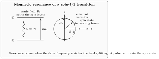
A static field $B_0$ creates a spin transition frequency $\omega_0$. A transverse oscillating field $B_1(t)$ near $\omega_0$ drives coherent transitions; pulse duration and detuning determine the rotation in the effective two-level system.

Resonant Transitions

To drive the spin, apply a weak transverse oscillating field. A schematic field is

$$\mathbf B(t) = B_0\hat{\mathbf z} + B_1\cos(\omega t)\hat{\mathbf x}.$$

The transverse part couples the two spin projections because it contains $S_x$. The system responds strongly when

$$\omega \simeq \omega_0.$$

Near resonance, and under the usual weak-drive assumptions, the rotating-wave approximation turns the driven problem into an effective two-level Hamiltonian. In a common rotating-frame convention,

$$H_{\mathrm{eff}} = \frac{\hbar}{2} \left( \Delta\sigma_z+\Omega\sigma_x \right),$$

where

$$\Delta=\omega_0-\omega.$$

The parameter $\Omega$ is the drive strength in angular-frequency units. Its exact relation to $B_1$ depends on whether the transverse field is linearly or circularly polarized and on the convention used in the Hamiltonian. For a resonant circularly rotating field one often has $\Omega=\lvert\gamma\rvert B_1$; a linearly oscillating field contains two rotating components, only one of which is resonant in the rotating-wave approximation.

On resonance, a pulse of duration $t$ rotates the two-level state by an angle

$$\theta = \Omega t.$$

A $\pi$ pulse flips population between the two spin projections. A $\pi/2$ pulse creates a coherent superposition. Those pulse ideas became central in nuclear magnetic resonance, electron spin resonance, atomic clocks, quantum optics, and quantum information.

Molecular Beam Resonance

The earliest magnetic-resonance program was closely tied to molecular and atomic beams. In the molecular beam magnetic-resonance method, particles pass through magnetic-field regions that select, drive, and analyze internal magnetic states. When the applied radio-frequency field matches an internal transition frequency, the beam intensity at a detector changes.

This was a major step beyond passive magnetic deflection. A Stern–Gerlach apparatus separates components; a resonance apparatus can induce transitions between them. It therefore measures magnetic moments through frequencies rather than only through spatial deflections. Frequency measurement is extraordinarily precise, so magnetic resonance turned small magnetic moments and hyperfine splittings into precision observables.

Historically, this route led to accurate nuclear magnetic moments, hyperfine structure measurements, and later atomic-clock methods. It also made the connection between magnetic moments and quantum transitions operational:

$$\hbar\omega = E_f-E_i.$$

The same equation appears in spectroscopy, but magnetic resonance made the controlled transition itself the instrument.

Nuclear Magnetic Resonance

Nuclear magnetic resonance, or NMR, uses transitions of nuclear magnetic moments in a magnetic field. A nucleus with nonzero spin has magnetic sublevels. A radio-frequency field can drive transitions between them when the frequency matches the Larmor frequency.

For a spin-$1/2$ nucleus,

$$\frac{\omega_0}{2\pi} = \left( \frac{\gamma}{2\pi} \right) B_0.$$

For protons,

$$\frac{\gamma_p}{2\pi} \approx 42.58\,\mathrm{MHz/T}.$$

Real NMR is richer than the isolated-spin formula. Chemical shielding shifts the local field and therefore the resonance frequency. Spin-spin couplings split lines. Relaxation times $T_1$ and $T_2$ describe return to thermal equilibrium and loss of transverse coherence. Pulse sequences can refocus inhomogeneous dephasing, select coherences, and measure structure.

For quantum mechanics, NMR is important because it turns abstract spin precession into a controllable laboratory language. It also teaches a recurring lesson: spectra, dynamics, and environment must be modeled together.

Electron Spin Resonance

Electron spin resonance, also called electron paramagnetic resonance, drives transitions of unpaired electron spins. Because the electron magnetic moment is much larger than a nuclear magnetic moment, electron resonance frequencies are much higher at the same field.

A useful scale is

$$\frac{\lvert\gamma_e\rvert}{2\pi} \approx 28.0\,\mathrm{GHz/T}$$

for a nearly free electron with $g\simeq2$. Thus a microwave frequency near $9.5\,\mathrm{GHz}$ corresponds to a field near $0.34\,\mathrm T$.

Electron spin resonance is sensitive to $g$ factors, local crystal fields, hyperfine coupling to nearby nuclei, exchange interactions, and spin relaxation. It became a central tool in chemistry, condensed matter, radiation damage studies, defects in solids, and spin-based quantum technologies.

The same caution applies as in the Zeeman effect: there is no universal resonance formula without specifying the effective Hamiltonian. A free electron, an electron in a molecule, a defect center in a crystal, and an effective spin in a many-body material can have different $g$ tensors and couplings.

Measuring Magnetic Moments

Magnetic resonance measures magnetic moments by comparing a transition frequency with a calibrated magnetic field. The simplest proportionality is

$$\omega_0 = \lvert\gamma\rvert B_0.$$

If $B_0$ is known, measuring $\omega_0$ determines $\lvert\gamma\rvert$. With the angular momentum known, this gives a magnetic moment or $g$ factor.

In practice, precision work must control:

• magnetic-field calibration and homogeneity;
• line broadening from field gradients and interactions;
• power broadening from strong drives;
• systematic shifts from neighboring levels;
• relaxation and decoherence;
• sample geometry and environmental couplings.

That list is not a nuisance added after the “real” quantum mechanics. It is part of the quantum experiment. The frequency being measured belongs to an effective Hamiltonian embedded in a real apparatus.

Quantum Control Preview

Magnetic resonance supplied much of the vocabulary of coherent control:

• resonant pulses;
• detuning;
• rotating frames;
• $\pi$ pulses and $\pi/2$ pulses;
• Ramsey sequences;
• spin echoes;
• relaxation and dephasing times;
• tomography-like reconstruction of spin components.

Those ideas later reappeared across quantum optics, trapped ions, superconducting circuits, nitrogen-vacancy centers, semiconductor spins, and other platforms. The hardware changed, but the two-level control logic remained recognizable.

The historical lesson is therefore broader than a particular technique. Magnetic resonance showed that quantum states could be manipulated coherently and reproducibly, not only inferred from static spectra.

Common Mistakes

• Forgetting that the sign of the gyromagnetic ratio matters.
• Treating $\Omega=\gamma B_1$ as universal without stating polarization and convention.
• Confusing Larmor precession in a static field with resonant population transfer from a transverse drive.
• Assuming every resonance line identifies one isolated spin without checking interactions and broadening.
• Ignoring relaxation and dephasing when interpreting line widths or pulse experiments.
• Treating NMR and ESR as purely classical signal-processing techniques; the measured frequencies and transitions come from quantum energy splittings.
• Overstating coherent control: good pulses require calibration, bandwidth control, and an effective two-level approximation.

Cross-Links

• Experimental Techniques and Instruments
• Stern–Gerlach Experiment
• Magnetic Moments
• Electron Spin
• Zeeman Effect
• Spin in Magnetic Fields
• Larmor Precession
• Magnetic Resonance Overview
• Spin in Magnetic Field Hamiltonian
• Rabi Oscillations: First Encounter
• Rotating-Wave Approximation
• Time-Dependent Hamiltonians
• Bloch Sphere

References

• I. I. Rabi, S. Millman, P. Kusch, and J. R. Zacharias, “The Molecular Beam Resonance Method for Measuring Nuclear Magnetic Moments,” Physical Review 55, 526-535, 1939, DOI: 10.1103/PhysRev.55.526.
• F. Bloch, “Nuclear Induction,” Physical Review 70, 460-474, 1946, DOI: 10.1103/PhysRev.70.460.
• E. M. Purcell, H. C. Torrey, and R. V. Pound, “Resonance Absorption by Nuclear Magnetic Moments in a Solid,” Physical Review 69, 37-38, 1946, DOI: 10.1103/PhysRev.69.37.
• A. Abragam, The Principles of Nuclear Magnetism, Oxford University Press, 1961.
• C. P. Slichter, Principles of Magnetic Resonance, 3rd ed., Springer, 1990.
• C. P. Poole Jr., Electron Spin Resonance: A Comprehensive Treatise on Experimental Techniques, 2nd ed., Dover, 1996.
• M. H. Levitt, Spin Dynamics: Basics of Nuclear Magnetic Resonance, 2nd ed., Wiley, 2008.

Exercises

1. Estimate the proton NMR frequency in a $3.0\,\mathrm T$ magnetic field using $\gamma_p/(2\pi)=42.58\,\mathrm{MHz/T}$.

Solution

Use

$$\frac{\omega_0}{2\pi} = \left( 42.58\,\mathrm{MHz/T} \right) B_0.$$

For $B_0=3.0\,\mathrm T$,

$$\frac{\omega_0}{2\pi} \approx 127.7\,\mathrm{MHz}.$$

2. A nearly free electron has $\lvert\gamma_e\rvert/(2\pi)\approx28.0\,\mathrm{GHz/T}$. What field corresponds to an ESR frequency of $9.5\,\mathrm{GHz}$?

Solution

Solve $f=(\lvert\gamma_e\rvert/2\pi)B_0$:

$$B_0 = \frac{9.5\,\mathrm{GHz}}{28.0\,\mathrm{GHz/T}} \approx 0.34\,\mathrm T.$$

3. If an on-resonance drive has Rabi frequency $\Omega/(2\pi)=25\,\mathrm{kHz}$, what is the duration of a $\pi$ pulse?

Solution

A $\pi$ pulse satisfies $\Omega t_\pi=\pi$, so

$$t_\pi = \frac{\pi}{\Omega} = \frac{1}{2(25\,\mathrm{kHz})} = 20\,\mu\mathrm s.$$

4. Why must the resonant driving field have a transverse component?

Solution

For a static field along $z$, the energy eigenstates are eigenstates of $S_z$. A field parallel to $z$ mostly shifts the level energies because it is diagonal in that basis. A transverse field contains $S_x$ or $S_y$, which has off-diagonal matrix elements between the two spin projections and can drive transitions.