Atomic Beams

Atomic beam experiments send atoms or molecules through a low-pressure apparatus so that their internal states can be prepared, deflected, driven, and detected with controlled fields. They made quantum discreteness visible in the Stern–Gerlach Experiment and later made precision magnetic-resonance and clock measurements possible.

This page treats atomic beams as an experimental platform. It does not replace the canonical spin formalism, spectroscopy, or time-dependent perturbation theory. For those, see What Spin Is and Is Not, Magnetic Resonance, and Selection Rules and Transition Rates.

Why Atomic Beams Matter

An atomic beam turns a hot gas or source into a directed stream of particles. That sounds simple, but it changed what could be measured. A beam experiment can separate preparation, interaction, and detection into different regions of space:

source -> collimation -> state selection -> interaction -> analyzer -> detector

This separation made several quantum ideas experimentally sharp:

• field gradients could turn magnetic-moment projections into spatial deflections;
• oscillating fields could drive transitions between internal states;
• interaction time could be controlled by beam speed and apparatus length;
• detected intensity could be used as a proxy for state population;
• vacuum reduced random collisions that would otherwise scramble the beam.

Atomic beams therefore sit between spectroscopy and modern quantum control. They keep the particles moving, but they give the experimenter enough control to ask state-resolved questions.

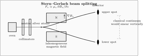
The Stern–Gerlach apparatus is an atomic-beam experiment: an oven produces neutral atoms, collimators define the beam, an inhomogeneous magnetic field separates magnetic-moment projections, and a detector records the output.

Sources and Collimation

Early atomic beams often began with a heated oven. Atoms escaped through a small aperture into a low-pressure region. The source was not a laser-cooled point source; it had a thermal velocity distribution and a finite angular spread.

For a thermal source, a characteristic speed scale is

$$v_{\rm th} \sim \sqrt{\frac{k_BT}{m}}.$$

The flux distribution from an effusive oven weights faster particles more strongly than the distribution inside the oven. The details matter in precision work, but the first lesson is enough here: a beam contains a range of velocities unless a velocity selector or cooling method narrows it.

Collimating slits reduce angular spread. If a slit of width $w$ is separated from a second aperture or interaction region by a distance $L$, a simple angular scale is

$$\theta_{\rm coll} \sim \frac{w}{L}.$$

Narrower collimation gives better angular definition but lower intensity. That tradeoff appears throughout beam physics: better state resolution usually costs signal rate.

Magnetic and Electric Fields

Neutral atoms are not deflected by the ordinary Lorentz force on net charge, but their internal magnetic and electric moments can couple to field gradients. In a simple magnetic-gradient geometry,

$$F_z \simeq \mu_z \frac{\partial B_z}{\partial z}.$$

This is the mechanism behind Stern–Gerlach separation. The apparatus converts a magnetic-moment projection into a position on a detector.

Electric fields play analogous roles when atoms or molecules have electric dipole moments, polarizabilities, or Stark shifts. The relevant force depends on the energy shift:

$$\mathbf F = - \boldsymbol\nabla E_{\rm internal}(\mathbf r).$$

The field does not need to reveal a little classical arrow. It couples to a quantum level structure. In weak fields one may label states by approximate angular-momentum quantum numbers; in strong or mixed fields those labels can change, and the effective Hamiltonian must be specified.

State Selection and Analysis

Atomic beam experiments often use field gradients twice. The first inhomogeneous field selects a sub-beam associated with particular internal states. A middle region then perturbs the selected atoms. A final analyzer converts internal-state changes back into a spatial or intensity change.

This logic underlies molecular beam resonance:

1. Prepare a beam and select a state component.
2. Apply an oscillating field in a controlled region.
3. Drive transitions when $\hbar\omega$ matches an internal energy difference.
4. Analyze the outgoing state population by magnetic deflection or intensity.

The detected signal is often a dip, peak, or fringe in beam intensity as a function of drive frequency. The observable is macroscopic, but the interpretation is quantum: the beam intensity depends on transition probabilities between internal states.

Velocity and Transit Time

The time an atom spends in an interaction region matters. If a beam with speed $v$ crosses a field region of length $\ell$, then

$$T \simeq \frac{\ell}{v}.$$

This transit time sets a Fourier-limited frequency scale:

$$\Delta\nu \sim \frac{1}{T}.$$

Longer interaction times give narrower resonances, all else equal. But slow beams can be harder to produce, more sensitive to stray fields, and more affected by collisions or gravity. Beam design is therefore a balance among intensity, velocity spread, interaction time, and systematic effects.

Ramsey’s separated-oscillatory-field method improved frequency resolution by using two separated interaction regions. The phase accumulated between them produces fringes whose spacing is set by the free evolution time. This is one of the bridges from atomic beams to atomic clocks.

Precision Measurement

Atomic beams became precision tools because they turned small energy differences into frequencies. Frequencies can be compared, counted, and stabilized with extraordinary accuracy.

Examples include:

• measuring nuclear magnetic moments with molecular beam resonance;
• measuring hyperfine splittings in atoms;
• testing Zeeman and Stark shifts;
• refining magnetic moments and $g$ factors;
• developing beam clocks and frequency standards;
• measuring scattering cross sections and interaction potentials with controlled beams.

The power of the method is also its weakness: the experimenter must understand the apparatus well enough to separate the desired level shift from systematic shifts. Magnetic-field gradients, stray electric fields, blackbody radiation, collisions, finite beam geometry, velocity distributions, and detector response can all matter.

Bridge to Modern AMO Physics

Modern atomic, molecular, and optical physics often uses trapped atoms, laser-cooled samples, optical lattices, and ion traps rather than hot effusive beams. Still, the beam tradition remains visible.

The conceptual descendants include:

• Stern–Gerlach state analysis in spin experiments;
• Ramsey interferometry in clocks and qubits;
• Rabi pulses for coherent state control;
• molecular beams for collision studies and precision spectroscopy;
• atom interferometers that use beam splitters and phase accumulation;
• supersonic beams and buffer-gas beams for cold-molecule preparation.

The historical continuity is important. Atomic beams showed that quantum internal states could be prepared, manipulated, and analyzed in a reproducible apparatus. That is a central idea of modern quantum experiments.

Common Mistakes

• Treating an atomic beam as a collection of identical particles all moving at one speed.
• Forgetting that collimation improves angular definition at the cost of intensity.
• Confusing a state selector with a passive filter that simply reveals pre-existing classical orientations.
• Ignoring field inhomogeneity, which is essential for Stern–Gerlach deflection.
• Assuming beam intensity directly equals a transition probability without accounting for apparatus acceptance.
• Treating resonance linewidths as purely natural linewidths; transit time, field gradients, and velocity spread often dominate.
• Reading atomic beam results without specifying the effective Hamiltonian and state labels used in the field regime.

Cross-Links

• Experimental Techniques and Instruments
• Stern–Gerlach Experiment
• Space Quantization
• Magnetic Moments
• Magnetic Resonance
• Spectroscopy
• Zeeman Effect
• Stark Effect
• Selection Rules and Transition Rates
• Interferometry

References

• O. Stern, “Ein Weg zur experimentellen Prüfung der Richtungsquantelung im Magnetfeld,” Zeitschrift für Physik 7, 249-253, 1921.
• W. Gerlach and O. Stern, “Der experimentelle Nachweis der Richtungsquantelung im Magnetfeld,” Zeitschrift für Physik 9, 349-352, 1922, DOI: 10.1007/BF01326983.
• I. I. Rabi, S. Millman, P. Kusch, and J. R. Zacharias, “The Molecular Beam Resonance Method for Measuring Nuclear Magnetic Moments,” Physical Review 55, 526-535, 1939, DOI: 10.1103/PhysRev.55.526.
• N. F. Ramsey, Molecular Beams, Oxford University Press, 1956.
• B. Friedrich and D. Herschbach, “Stern and Gerlach: How a Bad Cigar Helped Reorient Atomic Physics,” Physics Today 56, 53-59, 2003, DOI: 10.1063/1.1650229.
• H. Pauly, Atom, Molecule, and Cluster Beams I: Basic Theory, Production and Detection of Thermal Energy Beams, Springer, 2000.
• C. J. Foot, Atomic Physics, Oxford University Press, 2005.

Exercises

1. A collimating slit has width $w=0.20\,\mathrm{mm}$ and is followed by an interaction region $L=0.50\,\mathrm m$ away. Estimate the angular spread scale $\theta_{\rm coll}$.

Solution

Use $\theta_{\rm coll}\sim w/L$:

$$\theta_{\rm coll} \sim \frac{2.0\times10^{-4}\,\mathrm m}{0.50\,\mathrm m} = 4.0\times10^{-4}\,\mathrm{rad}.$$

2. A beam travels at $v=800\,\mathrm{m/s}$ through an interaction region of length $\ell=0.20\,\mathrm m$. Estimate the transit time and the scale $1/T$.

Solution

The transit time is

$$T \simeq \frac{\ell}{v} = \frac{0.20}{800}\,\mathrm s = 2.5\times10^{-4}\,\mathrm s.$$

The corresponding frequency scale is

$$\frac{1}{T} \simeq 4.0\,\mathrm{kHz}.$$

3. Why did neutral atoms help the Stern–Gerlach experiment isolate magnetic-moment physics?

Solution

A charged beam in a magnetic field experiences a Lorentz force depending on charge and velocity. Neutral atoms avoid that dominant charge deflection. Their magnetic moments can still couple to a field gradient, so the apparatus can separate components according to magnetic-moment projection rather than ordinary charge motion.

4. In a resonance beam experiment, why is a final analyzer needed after the oscillating-field region?

Solution

The oscillating field changes internal-state populations, but the detector usually measures beam intensity or position. A final analyzer converts internal state information into a detectable spatial or intensity difference. Without that analyzer, a transition may occur without producing an easily distinguishable signal.