Interferometry

Interferometry is the art of splitting a wave or quantum amplitude into alternatives, letting those alternatives accumulate relative phase, and recombining them so that phase becomes an observable intensity, count rate, or fringe displacement. It is one of the most important experimental languages of quantum mechanics because it makes phase measurable without treating phase itself as a directly displayed object.

This page explains interferometry as a technique family. The classical wave background is reviewed in Classical Waves and Interference. Matter-wave platforms are surveyed in Interference With Matter. The formal probability rule belongs to Probability Amplitudes and Born Rule.

The quantum-optical Mach–Zehnder unitary, coherent shot-noise baseline, and squeezed-input phase readout are developed at Interferometers.

Interferometer Logic

An interferometer has four conceptual parts:

• a coherent source;
• a splitter that creates alternatives;
• a region where the alternatives acquire different phases;
• a recombiner and detector that convert relative phase into observed probabilities.

The simplest two-alternative amplitude rule is

$$A = A_1+A_2, \qquad P = \lvert A_1+A_2\rvert^2.$$

Writing $A_j=\lvert A_j\rvert e^{i\phi_j}$ gives

$$\begin{aligned} P = {}& \lvert A_1\rvert^2 + \lvert A_2\rvert^2 \\ &+ 2\lvert A_1\rvert\lvert A_2\rvert \cos(\phi_2-\phi_1). \end{aligned}$$

The last term is the interference term. It is the reason an interferometer can measure a small path change, potential change, acceleration, rotation, refractive-index change, magnetic flux, or gravitational phase shift. The device translates a phase difference into a count-rate difference.

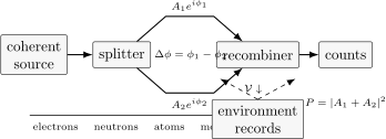
Interferometers share a common logic even when the hardware differs: prepare coherence, split amplitudes, accumulate relative phase, recombine, and read out counts. Environmental records reduce visibility because they make the alternatives distinguishable.

Optical Interferometers

Classical optical interferometers were essential before quantum mechanics. They established a mature laboratory grammar for phase, coherence, path difference, and fringe visibility. Later quantum experiments inherited that grammar but changed the interpretation of weak beams and single detection events.

In a simple optical two-beam interferometer, a path-length difference $\Delta L$ produces phase

$$\Delta\phi = \frac{2\pi}{\lambda}\Delta L,$$

for wavelength $\lambda$ in the relevant medium. A common fringe model is

$$I(\Delta\phi) = I_{\rm avg} \left[ 1+\mathcal V\cos(\Delta\phi+\phi_0) \right],$$

where $\mathcal V$ is the visibility and $\phi_0$ is a fixed offset from the instrument. In a balanced ideal interferometer $\mathcal V$ approaches $1$. In a real instrument it is reduced by unequal intensities, finite bandwidth, source size, vibration, polarization mismatch, detector averaging, and uncontrolled environmental phase noise.

Familiar optical designs include Michelson, Mach–Zehnder, Fabry–Perot, Sagnac, and Ramsey-style separated-field arrangements. Their hardware differs, but each makes a relative phase observable. A Michelson interferometer is naturally sensitive to path length. A Sagnac interferometer is naturally sensitive to rotation. A Fabry–Perot cavity enhances phase sensitivity by multiple passes and resonant buildup.

The two-pulse unitary, finite-pulse fringes, detuning estimators, and clock feedback application are developed in Ramsey Interferometry.

For quantum mechanics, the key lesson is not that light is merely a classical wave. The same optical apparatus can be operated at low intensity, where detections occur one by one. The accumulated counts still follow the interference probabilities. This is why interferometry is a bridge between classical wave optics and quantum probability amplitudes.

Beam Splitters as Amplitude Devices

A beam splitter should be understood as a device that transforms input amplitudes into output amplitudes. In an ideal two-port model, one may write schematically

$$\begin{pmatrix} a_{\rm out} \\ b_{\rm out} \end{pmatrix} = U \begin{pmatrix} a_{\rm in} \\ b_{\rm in} \end{pmatrix},$$

where $U$ is a unitary matrix when loss is neglected. Different phase conventions are possible. The physics is in the relative phases and in the fact that amplitudes, not probabilities, are recombined.

For a balanced interferometer with one input and two alternatives of equal magnitude, a detector probability often has the form

$$P_+ = \frac{1}{2} \left[ 1+\cos\Delta\phi \right], \qquad P_- = \frac{1}{2} \left[ 1-\cos\Delta\phi \right].$$

These two outputs are complementary. When one is bright, the other is dark. In photon-counting language this means count rates are redistributed between detectors, not that energy is created by constructive interference or destroyed by destructive interference.

This point is easy to miss. Interference changes probabilities at output ports because amplitudes from alternatives add with phase. It does not mean each particle splits into two classical half-particles that later collide.

Phase Sensitivity

Interferometers are phase meters. Near a point where the output changes rapidly with phase, a small phase shift $\delta\phi$ produces a measurable count-rate change. If

$$P(\phi) = \frac{1}{2} \left[ 1+\mathcal V\cos\phi \right],$$

then

$$\frac{dP}{d\phi} = - \frac{\mathcal V}{2}\sin\phi.$$

The largest slope occurs near $\phi=\pi/2$ or $3\pi/2$, so interferometers are often operated near quadrature rather than at a maximum or minimum.

For independent detection events, counting noise typically scales like $1/\sqrt N$ for $N$ detected quanta under ordinary conditions. This standard quantum limit is not the final word in quantum metrology, but it is the baseline expectation. Squeezed states, entangled probes, and adaptive measurements can improve particular measurement tasks, subject to loss and technical noise. Those refinements belong to quantum optics and quantum information; the historical technique lesson is simply that phase sensitivity is statistical as well as optical.

Matter-Wave Interferometers

Matter-wave interferometers apply the same amplitude logic to electrons, neutrons, atoms, and molecules. The relevant wavelength is not an optical wavelength but the de Broglie wavelength

$$\lambda = \frac{h}{p}.$$

The alternatives may be created by crystal diffraction, electrostatic biprisms, material gratings, standing light waves, Raman pulses, Bragg pulses, or other coherent devices. During propagation, the phase can often be written semiclassically as an action phase,

$$\phi = \frac{S}{\hbar},$$

so a difference in action gives

$$\Delta\phi = \frac{S_1-S_2}{\hbar}.$$

Different platforms make different phases accessible:

Platform	Common splitting method	Example phase sensitivity
electrons	crystal diffraction, biprisms, nanostructures	electromagnetic potentials, material interactions, enclosed magnetic flux
neutrons	perfect-crystal Bragg diffraction	gravity, rotation, magnetic fields, nuclear scattering phases
atoms	material gratings, standing waves, Raman or Bragg pulses	acceleration, rotation, gravity gradients, internal-state phases
molecules	near-field gratings, optical gratings, time-domain gratings	polarizability, decoherence, environmental phase noise

The matter-wave lesson is especially important historically. Interference is not tied to a classical electromagnetic field. Massive particles can also carry phase, and localized detections can accumulate into an interference pattern. For the broader matter-wave story, see Interference With Matter. The platform-level Raman and Bragg pulse sequence, acceleration and rotation phases, closure, and calibration ledger are developed in Atom Interferometry.

Which-Way Information

Interference requires coherent alternatives that remain indistinguishable in the relevant physical state. If a detector, environment, internal state, or scattered photon records which path was taken, the interference term is reduced.

A compact model attaches detector states to the two alternatives:

$$\lvert\Psi\rangle = A_1\lvert 1\rangle\lvert D_1\rangle + A_2\lvert 2\rangle\lvert D_2\rangle.$$

If the detector record is ignored, the observed interference contains the overlap $\langle D_1|D_2\rangle$:

$$\begin{aligned} P = {}& \lvert A_1\rvert^2 + \lvert A_2\rvert^2 \\ &+ 2\operatorname{Re} \left[ A_1^*A_2 \langle D_1|D_2\rangle \right]. \end{aligned}$$

If $\langle D_1|D_2\rangle=1$, the detector states are identical and full interference is possible. If $\langle D_1|D_2\rangle=0$, the path records are perfectly distinguishable and the interference term vanishes.

This is more precise than saying “observing destroys the wave.” What matters is physical distinguishability and entanglement with records. A person looking is not the essential ingredient. The essential ingredient is whether information about the alternative has become available in the physical state.

Quantum Metrology Preview

Interferometry became one of the main routes from foundational quantum evidence to precision measurement. The same phase sensitivity that makes interference conceptually sharp also makes it technologically powerful.

Examples include:

• optical interferometry for displacement, refractive-index, rotation, and gravitational-wave measurements;
• neutron interferometry for gravitational and magnetic quantum phases;
• atom interferometry for accelerometry, gravimetry, gyroscopes, and tests of inertial effects;
• Ramsey interferometry for atomic clocks and spectroscopy;
• superconducting and mesoscopic interferometers for magnetic flux and phase coherence.

This preview should not be read as a claim that every interferometer is “more quantum” than every non-interferometric instrument. The quantum content depends on the state preparation, detection regime, noise model, and control of coherence. Interferometry is powerful because it gives a precise operational handle on phase.

Common Mistakes

• Treating phase as a directly visible substance rather than an inferred quantity from interference.
• Adding probabilities where amplitudes should be added.
• Assuming any two paths interfere even when which-way information is present.
• Forgetting that visibility can be reduced by mundane imperfections as well as by fundamental decoherence.
• Interpreting dark-port destructive interference as destruction of energy rather than redistribution among output modes.
• Treating matter-wave interference as a statement that particles are ordinary classical waves.
• Overstating quantum metrology: entanglement and squeezing can help, but loss, noise, and calibration decide practical performance.

Cross-Links

• Quantum Optical Interferometers
• Ramsey Interferometry
• Experimental Techniques and Instruments
• Classical Waves and Interference
• Double-Slit Experiment
• Interference With Matter
• de Broglie Matter Waves
• Probability Amplitudes
• Born Rule
• Superposition and Relative Phase
• Decoherence Preview
• Berry Phase

References

• M. Born and E. Wolf, Principles of Optics, 7th expanded ed., Cambridge University Press, 1999.
• L. Mandel and E. Wolf, Optical Coherence and Quantum Optics, Cambridge University Press, 1995.
• Y. Aharonov and D. Bohm, “Significance of Electromagnetic Potentials in the Quantum Theory,” Physical Review 115, 485-491, 1959, DOI: 10.1103/PhysRev.115.485.
• R. Colella, A. W. Overhauser, and S. A. Werner, “Observation of Gravitationally Induced Quantum Interference,” Physical Review Letters 34, 1472-1474, 1975, DOI: 10.1103/PhysRevLett.34.1472.
• H. Rauch and S. A. Werner, Neutron Interferometry: Lessons in Experimental Quantum Mechanics, 2nd ed., Oxford University Press, 2015.
• P. R. Berman, ed., Atom Interferometry, Academic Press, 1997.
• A. D. Cronin, J. Schmiedmayer, and D. E. Pritchard, “Optics and Interferometry with Atoms and Molecules,” Reviews of Modern Physics 81, 1051-1129, 2009, DOI: 10.1103/RevModPhys.81.1051.

Exercises

1. A Michelson-style interferometer uses light of wavelength $\lambda=633\,\mathrm{nm}$. What phase shift is produced by a path-length change $\Delta L=100\,\mathrm{nm}$?

Solution

Use

$$\Delta\phi = \frac{2\pi}{\lambda}\Delta L.$$

Thus

$$\Delta\phi = 2\pi \frac{100}{633} \approx 0.99\,\mathrm{rad}.$$

2. For $A_1=A_2=A_0e^{i\phi_j}$, show that the probability is proportional to $1+\cos\Delta\phi$.

Solution

Let $\Delta\phi=\phi_2-\phi_1$. Then

$$\begin{aligned} \lvert A_1+A_2\rvert^2 &= \lvert A_0\rvert^2 \lvert e^{i\phi_1}+e^{i\phi_2}\rvert^2 \\ &= 2\lvert A_0\rvert^2 \left[ 1+\cos\Delta\phi \right]. \end{aligned}$$

The overall normalization depends on the beam-splitter convention, but the phase dependence is $1+\cos\Delta\phi$.

3. In the which-way model, what happens to interference if $\langle D_1|D_2\rangle=0$?

Solution

The detector states are orthogonal, so the alternatives are perfectly distinguishable in principle. The interference term is multiplied by zero and disappears from the reduced probability. The result is the incoherent sum $\lvert A_1\rvert^2+\lvert A_2\rvert^2$.

4. Why is operating near quadrature useful for phase measurement?

Solution

For

$$P(\phi) = \frac{1}{2} \left[ 1+\mathcal V\cos\phi \right],$$

the slope is

$$\frac{dP}{d\phi} = - \frac{\mathcal V}{2}\sin\phi.$$

Near $\phi=\pi/2$ or $3\pi/2$, the magnitude of the slope is maximal, so a small phase change produces the largest first-order change in output probability.