Ramsey Interferometry

Ramsey interferometry converts phase accumulated by a coherent superposition into a measurable population. A first pulse divides amplitude between two internal states, the components evolve freely, and a second pulse recombines them. The resulting population oscillates with detuning, free-evolution time, or pulse phase.

For ideal instantaneous $\pi/2$ pulses, an atom prepared in $|g\rangle$ has

$$\begin{aligned} P_e &= \frac12 \left[ 1+\cos\Phi \right], \\ \Phi &= \Delta T+\phi_1-\phi_2, \\ \Delta &\equiv \omega_0-\omega_L. \end{aligned}$$

Here $T$ is the free-evolution interval and $\phi_1,\phi_2$ are the phases of the two pulses in a common rotating-frame convention. The formula is simple; using it as a precision measurement requires careful control of pulse area, finite pulse duration, phase references, readout, decoherence, oscillator noise, and shifts of the atomic transition.

Ramsey’s original method used two interaction zones separated in space. Modern implementations often use two pulses separated in time. The interference principle is the same in both cases.

Canonical Scope

This page owns the AMO separated-field measurement ledger:

1. the two-pulse unitary and its phase conventions;
2. arbitrary pulse-area contrast and offset;
3. ideal and finite-pulse Ramsey fringes;
4. fringe spacing, central-fringe width, and capture range;
5. detuning estimators and phase-stepped error signals;
6. the feedback logic of passive atomic clocks;
7. experiment-facing noise and systematic-phase diagnostics.

Neighboring pages have distinct canonical roles:

• Ramsey Interferometry for Quantum Estimation owns the binary likelihood, Fisher information, working-point and interrogation-time design, phase unwrapping, and matched sensing claims.
• Two-Level Atom owns the reduction from a multilevel spectrum to the driven two-state Hamiltonian and the detuning convention used here.
• Rabi Oscillations owns drive-strength calibration, pulse area, Rabi traces, chevrons, and readout diagnostics.
• Time-Dependent Two-Level Systems Notebook owns the executable ideal-versus-finite pulse comparison and phase-stepped Ramsey benchmark, together with its numerical validation record.
• Rabi and Ramsey Control owns the protocol-level comparison of Rabi, Ramsey, echo, and dynamical decoupling in open systems.
• Decoherence Timescales owns the distinction among $T_1$, $T_2$, $T_2^*$, and echo coherence.
• Precision Spectroscopy owns uncertainty budgets, traceability, frequency ratios, and broader clock metrology.
• Interferometry owns the historical and cross-platform interferometer picture.

The purpose here is to connect a controlled two-state Hamiltonian to the actual observable that makes separated-field spectroscopy useful.

Conventions and Interferometer Logic

Take

$$\begin{aligned} \sigma_z|e\rangle &= |e\rangle, \\ \sigma_z|g\rangle &= -|g\rangle, \end{aligned}$$

and use the rotating-wave Hamiltonian

$$H_{\mathrm{RWA}} = \frac{\hbar}{2} \left( \Delta\sigma_z + \Omega\sigma_\phi \right),$$

where

$$\sigma_\phi = \cos\phi\,\sigma_x + \sin\phi\,\sigma_y.$$

This page takes $\Omega\ge0$. A sign in a matrix element can instead be absorbed into the drive phase $\phi$. Every quoted phase and detuning should be translated from the Hamiltonian before formulas from different sources are compared.

An internal-state interferometer

The two alternatives are amplitudes in $|g\rangle$ and $|e\rangle$:

prepare |g> -> split amplitudes -> accumulate relative phase
            -> recombine amplitudes -> measure an output population

This is interferometer logic even when the two components follow the same spatial trajectory. The phrase “two arms” then refers to two paths through Hilbert space, not necessarily two separated wave packets.

The first $\pi/2$ pulse plays the role of a balanced beam splitter. Free evolution supplies the differential phase. The second $\pi/2$ pulse is a phase-sensitive recombiner. Measuring $|e\rangle$ is analogous to counting one output port.

Pulse rotations

For a resonant pulse whose phase is constant, define

$$R_\phi(\theta) = \exp\!\left[ - \frac{i\theta}{2} \sigma_\phi \right],$$

with pulse area

$$\theta = \int_{\mathrm{pulse}} dt\,\Omega(t).$$

For a square pulse, $\theta=\Omega\tau$. Acting on the ground state,

$$R_\phi\!\left(\frac{\pi}{2}\right)|g\rangle = \frac{1}{\sqrt2} \left( |g\rangle - i e^{-i\phi}|e\rangle \right).$$

Equal populations alone do not define the state. The factor $-i e^{-i\phi}$ records the relative phase established by the drive.

The π/2 Pulse Sequence

First pulse: create coherence

Let the first pulse have phase $\phi_1$. Immediately after it,

$$|\psi_1\rangle = \frac{1}{\sqrt2} \left( |g\rangle - i e^{-i\phi_1}|e\rangle \right).$$

The state now has nonzero coherence $\rho_{ge}=\langle g|\rho|e\rangle$. Ramsey interferometry is sensitive to the phase of this off-diagonal matrix element.

Free evolution

With the drive absent, retain the rotating-frame detuning Hamiltonian

$$H_f = \frac{\hbar\Delta}{2}\sigma_z.$$

The free propagator is

$$U_f(T) = \exp\!\left( - \frac{i\Delta T}{2}\sigma_z \right).$$

Therefore

$$\begin{aligned} |\psi_f\rangle = \frac{1}{\sqrt2} \Bigl(& e^{i\Delta T/2}|g\rangle \\ &- i e^{-i\phi_1} e^{-i\Delta T/2}|e\rangle \Bigr). \end{aligned}$$

After removal of a global phase, the relative phase has advanced by $\Delta T$. A global phase cannot affect the final population; the difference between the two components can.

Second pulse: recombine

Apply a second $\pi/2$ pulse with phase $\phi_2$. The excited-state amplitude is the coherent sum of two alternatives:

1. amplitude transferred to $|e\rangle$ by the first pulse and retained by the second;
2. amplitude left in $|g\rangle$ by the first pulse and transferred by the second.

The result is

$$P_e = \frac12 \left[ 1+ \cos\!\left( \Delta T+\phi_1-\phi_2 \right) \right].$$

For equal pulse phases and zero detuning, the two $\pi/2$ rotations combine to a $\pi$ rotation and $P_e=1$. If the second phase differs by $\pi$, it undoes the first pulse and $P_e=0$. A phase shift of $\pi/2$ places the measurement at quadrature.

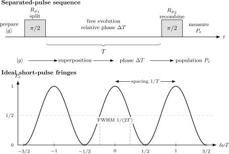
Top: the first $\pi/2$ pulse creates an internal-state superposition, free evolution for $T$ accumulates relative phase, and the second $\pi/2$ pulse maps that phase to population. Bottom: for ideal short pulses, scanning $\delta\nu=\Delta/(2\pi)$ gives fringes separated by $1/T$; the central fringe has FWHM $1/(2T)$.

Arbitrary pulse areas

In the ideal resonant-pulse limit, let the two areas be $\theta_1$ and $\theta_2$. Direct multiplication gives

$$\begin{aligned} P_e = \frac12 \Bigl[ 1 &- \cos\theta_1\cos\theta_2 \\ &+ \sin\theta_1\sin\theta_2 \cos\Phi \Bigr], \end{aligned}$$

where

$$\Phi = \Delta T+\phi_1-\phi_2.$$

The nonoscillating offset is

$$A = \frac12 \left( 1-\cos\theta_1\cos\theta_2 \right),$$

and the fringe amplitude is

$$B = \frac12 \sin\theta_1\sin\theta_2.$$

Balanced $\pi/2$ pulses maximize the ideal contrast. Pulse-area errors do not merely make the splitter “less efficient”: they change both the offset and the amplitude. Detuning during the pulses can additionally shift the fringe phase.

Phase is a control coordinate

The second pulse phase can be changed without changing the free-evolution time. At fixed $T$,

$$P_e(\phi_2) = \frac12 \left[ 1+ \cos\!\left( \Delta T+\phi_1-\phi_2 \right) \right].$$

A phase scan therefore measures the same accumulated coherence as a frequency or delay scan. It is often the cleanest way to place the interferometer at maximum slope.

Free Evolution and Phase Accumulation

Time-dependent detuning

If the transition or local oscillator changes during the dark time, replace $\Delta T$ by an integral:

$$\Phi = \int_0^T dt\, \Delta(t) + \phi_1-\phi_2.$$

With

$$\Delta(t) = \omega_0(t)-\omega_L(t),$$

the interferometer senses the time average

$$\overline\Delta = \frac{1}{T} \int_0^T dt\,\Delta(t).$$

One Ramsey result cannot say whether a phase came from the atom or the oscillator. The observable is their relative phase.

Atomic shifts and oscillator phase

Write

$$\begin{aligned} \omega_0(t) &= \omega_0^{(0)} + \delta\omega_a(t), \\ \omega_L(t) &= \omega_L^{(0)} + \delta\omega_L(t). \end{aligned}$$

Then

$$\begin{aligned} \Phi = {}& \left( \omega_0^{(0)}-\omega_L^{(0)} \right)T \\ &+ \int_0^T dt\, \left[ \delta\omega_a(t)-\delta\omega_L(t) \right] \\ &+ \phi_1-\phi_2. \end{aligned}$$

Magnetic, electric, collisional, motional, and blackbody shifts enter through $\delta\omega_a$. Laser or microwave phase noise enters through $\delta\omega_L$ and the pulse phases. A population trace alone does not separate them.

Bloch-sphere interpretation

The first pulse rotates the Bloch vector from the south pole to the equator. During free evolution, detuning rotates it around the $z$ axis. The second pulse projects one equatorial quadrature onto $z$.

At a fringe maximum the second pulse converts the accumulated phase into maximum excited population. At a fringe minimum it returns the atom to the ground state. At quadrature, a small phase change causes the largest population change.

The geometry is developed abstractly in Bloch Sphere. The present page keeps the link to measured frequency and pulse phase.

Spatially separated fields

For an atom moving at speed $v$ between interaction zones separated by distance $L$,

$$T = \frac{L}{v}.$$

The phase also includes the phase difference of the fields at the two interaction events. For a plane-wave component this can contain

$$\Delta\phi_{\mathrm{space}} = \mathbf k\mathbin{\cdot} \left( \mathbf r_2-\mathbf r_1 \right).$$

Velocity spread changes both $T$ and the sampled spatial phase. A molecular beam, thermal beam, fountain, trapped ion, and stationary optical-lattice ensemble therefore require different averaging models even when the two-level unitary is identical.

In an atomic fountain, atoms can pass through the same microwave cavity on the upward and downward trajectories. The long ballistic interval gives a narrow Ramsey pattern. Residual spatial phase variations of the cavity field can nevertheless produce a frequency shift.

Ramsey Fringes

Frequency scan

Define ordinary-frequency detuning

$$\delta\nu \equiv \frac{\Delta}{2\pi} = \nu_0-\nu_L.$$

For equal pulse phases,

$$P_e(\delta\nu) = \cos^2\!\left( \pi\delta\nu T \right).$$

Neighboring maxima satisfy

$$\Delta\nu_{\mathrm{fringe}} = \frac{1}{T}.$$

The nearest half-maximum points of the central fringe occur at

$$\left| \delta\nu \right| = \frac{1}{4T},$$

so its ideal short-pulse full width at half maximum is

$$\Delta\nu_{\mathrm{FWHM}} = \frac{1}{2T}.$$

This central feature is not a Lorentzian natural line. It is an interference fringe generated by a finite interrogation sequence.

Resolution and ambiguity

Longer $T$ narrows the central fringe and increases phase response:

$$\frac{\partial\Phi}{\partial\delta\nu} = 2\pi T.$$

The same change also places more fringes into a fixed search interval. A single measured population is periodic in phase and does not identify which fringe was observed.

Trustworthy acquisition often proceeds hierarchically:

1. use a short $T$ or independent spectroscopy to locate the resonance;
2. increase $T$ while keeping the estimated phase inside the capture range;
3. use phase stepping or measurements at several $T$ values;
4. unwrap phase only with an explicit continuity or prior-frequency model.

Narrower is not automatically more accurate. A narrow fringe can be shifted by a small systematic phase.

Broad envelope and narrow fringes

Real pulses have duration $\tau$. Their transition bandwidth is of order $1/\tau$, while the fine fringe spacing is of order $1/T$. When $T\gg\tau$, many Ramsey fringes lie beneath a broad pulse envelope.

This separates two scales:

pulse duration tau       broad excitation envelope
free interval T          narrow Ramsey fringe spacing

The Fourier and homogeneous width distinctions are treated in Line Shapes and Broadening.

Exact square-pulse expression

Consider two identical square pulses of duration $\tau$ and phase zero, with a field-free gap $T$ measured from the end of the first pulse to the start of the second. During each pulse,

$$H_p = \frac{\hbar}{2} \left( \Delta\sigma_z+\Omega\sigma_x \right).$$

Define

$$\begin{aligned} \Omega_R &= \sqrt{\Omega^2+\Delta^2}, \\ x &= \frac{\Omega_R\tau}{2}, \\ y &= \frac{\Delta T}{2}. \end{aligned}$$

The exact rotating-wave result is

$$\begin{aligned} P_e = {}& 4 \frac{\Omega^2}{\Omega_R^2} \sin^2x \\ &\times \left[ \cos x\cos y - \frac{\Delta}{\Omega_R} \sin x\sin y \right]^2. \end{aligned}$$

This formula includes detuning during the pulses. On exact resonance,

$$P_e(0) = \sin^2(\Omega\tau).$$

Thus two resonant pulses with $\Omega\tau=\pi/2$ produce complete excitation.

For such nominal square $\pi/2$ pulses and small detuning, the central phase behaves approximately as

$$\frac{\Delta T_{\mathrm{eff}}}{2},$$

with

$$\begin{aligned} T_{\mathrm{eff}} &\simeq T+\frac{2}{\Omega} \\ &= T+\frac{4\tau}{\pi}. \end{aligned}$$

The pulse contribution is negligible only when $T\gg\tau$. Quoting a linewidth without saying whether $T$ is edge-to-edge, center-to-center, or an effective sensitivity time can create avoidable factor-level disagreements.

Ramsey versus Rabi spectroscopy

A single square Rabi pulse and a Ramsey pair answer related but different questions.

• Rabi spectrum: one continuous interaction; width is set mainly by pulse duration and modified by coupling strength, damping, and shifts.
• Ramsey spectrum: two interactions separated by dark evolution; a broad pulse envelope contains narrow phase-interference fringes.
• Ramsey advantage: long phase accumulation need not require a strong field throughout the interval.
• Ramsey cost: phase coherence between the pulses and correct fringe identification become essential.

Rabi Oscillations owns the population-flopping calibration that normally precedes a Ramsey measurement.

Detuning Measurement

Operate at maximum slope

At a maximum or minimum of

$$P_e = \frac12 \left[ 1+C\cos\Phi \right],$$

the first derivative with respect to phase vanishes. Those points are good for checking contrast but poor for measuring a small phase change.

At quadrature,

$$\Phi = \frac{\pi}{2} \pmod{\pi},$$

and

$$\left| \frac{\partial P_e}{\partial\Phi} \right| = \frac{C}{2}.$$

The population response is then locally linear.

Phase-stepped error signal

Set $\phi_1=0$ and alternate the second-pulse phase between

$$\phi_2^{(\pm)} = \pm\frac{\pi}{2}.$$

The two probabilities are

$$\begin{aligned} P_+ &= \frac12 \left[ 1+C\sin(\Delta T) \right], \\ P_- &= \frac12 \left[ 1-C\sin(\Delta T) \right]. \end{aligned}$$

Their difference is an antisymmetric error signal:

$$\mathcal E \equiv P_+-P_- = C\sin(\Delta T).$$

Near lock,

$$\mathcal E \simeq C\Delta T.$$

The zero crossing identifies the chosen central fringe, and its slope converts population error into a frequency correction. Reversing the phase labels reverses the sign but not the information.

Side-of-fringe frequency modulation

Another method interrogates at frequencies

$$\nu_L = \nu_c\pm\nu_m$$

on opposite sides of a nominal center $\nu_c$. The difference in measured populations is driven toward zero by feedback.

This method assumes that the sampled line shape is symmetric about the desired unperturbed center. Asymmetric state preparation, power shifts, frequency chirps, cavity phase gradients, or detection changes correlated with the modulation can displace the servo zero.

Capture range

Near the central fringe, a simple unambiguous phase range is approximately

$$|\Delta T| \lesssim \frac{\pi}{2}.$$

Equivalently,

$$\left| \delta\nu \right| \lesssim \frac{1}{4T}.$$

Outside this region, the same population can correspond to multiple phase values. Feedback can lock to a neighboring fringe if the oscillator begins too far from the expected transition.

A fit model

For counts $k_j$ out of $N_j$ trials, a useful model is

$$k_j \sim \operatorname{Binomial} \left( N_j,p_j \right),$$

with

$$\begin{aligned} p_j &= A + B\,C(T_j) \cos\Theta_j, \\ \Theta_j &= 2\pi\delta\nu T_j \\ &\quad+ \phi_1-\phi_2 + \phi_{\mathrm{sys}}. \end{aligned}$$

The parameters have distinct meanings:

• $A$ is the baseline, including pulse and readout offsets;
• $B$ is the available contrast scale;
• $C(T)$ is the coherence envelope;
• $\delta\nu$ is the frequency detuning;
• $\phi_{\mathrm{sys}}$ is a fixed or modeled systematic phase.

One should not fit all of them freely to one short trace and expect a unique microscopic interpretation. Independent state-preparation and readout calibration, Rabi data, phase reversals, several values of $T$, and control experiments reduce degeneracy.

Fixed phase versus frequency shift

A systematic phase $\phi_{\mathrm{sys}}$ produces an apparent ordinary frequency bias of magnitude

$$\left| \delta\nu_{\mathrm{bias}} \right| = \frac{ |\phi_{\mathrm{sys}}| }{ 2\pi T }.$$

A phase localized to the pulses often gives a contribution that decreases approximately as $1/T$. A genuine shift acting throughout the dark time produces a phase proportional to $T$ and therefore a frequency bias that does not disappear at longer $T$. Measurements at several dark times can help distinguish these cases.

Atomic Clocks

What the clock actually is

A passive atomic clock is not merely an isolated atom “ticking.” It is a feedback system with at least four parts:

1. an atomic or ionic transition that supplies a reproducible frequency reference;
2. a local oscillator that generates a usable microwave or optical signal;
3. an interrogation and detection sequence that compares oscillator phase with atomic phase;
4. a servo that steers the oscillator from the measured error signal.

The output available to electronics and users is the disciplined local oscillator. The atoms provide the reference against which its long-term frequency is corrected.

Clock cycle

A simplified Ramsey clock cycle is:

prepare atoms
apply first pi/2 pulse
accumulate relative phase for T
apply phase-stepped second pi/2 pulse
measure population
form an error signal
update the local oscillator

Repeated cycles turn a probabilistic quantum measurement into a frequency estimate. State preparation, detection, and feedback dead time are part of the clock, not administrative details outside the physics.

The SI second

The current SI definition fixes the unperturbed ground-state hyperfine transition frequency of cesium-133 to

$$\Delta\nu_{\mathrm{Cs}} = 9\,192\,631\,770\ \mathrm{Hz}$$

exactly. This defines the second through a transition frequency, but a real primary standard must still realize the idealized unperturbed frequency by evaluating Zeeman, collisional, blackbody, Doppler, gravitational, and instrumental corrections.

Optical clocks use much higher transition frequencies and can achieve exceptional stability and systematic control, but the SI second remains defined by cesium as of this page’s review date. The current definition is maintained by the BIPM.

Atomic fountains

Laser-cooled cesium atoms in a fountain can traverse a microwave cavity on the way up and again on the way down. The two passages supply the separated interactions, while the ballistic flight supplies a long dark interval.

Compared with a thermal beam, slower atoms increase $T$ and narrow the Ramsey fringe. Fountain accuracy still depends on effects including:

• cold collisions;
• distributed cavity phase;
• microwave leakage;
• magnetic-field shifts;
• blackbody radiation;
• residual motion and recoil;
• state-selection and detection asymmetry.

The narrow fringe is only the discriminator. Accuracy comes from linking its servo zero to the specified unperturbed transition.

Optical clocks

Trapped ions and neutral atoms in optical lattices use narrow electronic transitions. Ramsey interrogation and composite variants are important, but single-pulse Rabi interrogation is also common. The best protocol depends on coherence, dead time, probe-induced shifts, particle number, available laser stability, and the transition.

A higher carrier frequency improves the spectroscopic quality factor

$$Q = \frac{\nu_0}{\Delta\nu},$$

but high $Q$ alone does not guarantee a low uncertainty. Readout noise, oscillator noise, atomic systematics, duty cycle, and reproducibility remain decisive.

Projection-noise scaling

For $N$ independent atoms measured at quadrature, the binomial population uncertainty is approximately

$$\sigma_P \simeq \frac{1}{2\sqrt N}.$$

The ideal Ramsey slope with respect to ordinary frequency is

$$\left| \frac{\partial P_e}{\partial\nu} \right| \simeq \pi C T.$$

One cycle then gives the order-of-magnitude frequency uncertainty

$$\sigma_\nu \simeq \frac{1}{ 2\pi C T\sqrt N }.$$

If independent cycles of duration $T_c$ are averaged for time $\tau_a$, the corresponding ideal fractional scaling is

$$\sigma_y(\tau_a) \simeq \frac{1}{ 2\pi\nu_0 C T\sqrt N } \sqrt{ \frac{T_c}{\tau_a} }.$$

This is a benchmark, not a universal clock formula. Entanglement can change the quantum scaling, while loss, dead time, technical noise, and estimator details can make performance worse.

Stability is not accuracy

• Stability describes fluctuations under repeated comparison and averaging.
• Accuracy or systematic uncertainty describes agreement between the realized frequency and the specified unperturbed transition.
• Resolution describes the ability of an interrogation to distinguish nearby frequencies.

A clock can have a narrow line but a shifted center, excellent short-term stability but a systematic bias, or low systematic uncertainty but slow averaging. These are different claims.

The full uncertainty and traceability framework belongs to Precision Spectroscopy.

Noise and Decoherence

A complex coherence factor

Let

$$\Delta(t) = \Delta_0+\xi(t),$$

where $\xi(t)$ is a stochastic relative-frequency fluctuation. Define

$$W(T) \equiv \left\langle \exp\!\left[ i\int_0^T dt\,\xi(t) \right] \right\rangle.$$

An idealized averaged fringe can be written

$$\begin{aligned} P_e(T) &= \frac12 \Bigl\{ 1+ \operatorname{Re} Z(T) \Bigr\}, \\ Z(T) &= W(T) e^{i\Phi_0}, \\ \Phi_0 &= \Delta_0T+\phi_1-\phi_2. \end{aligned}$$

The magnitude $|W(T)|$ is the coherence envelope. The argument $\arg W(T)$ is a noise-induced phase shift. Reducing every imperfection to a real positive contrast can hide a biased fringe center.

Markovian dephasing

For exponential transverse coherence decay,

$$W(T) = e^{-T/T_2}.$$

If population relaxation with time $T_1$ and Markovian pure dephasing rate $\gamma_\phi$ are the only channels,

$$\frac{1}{T_2} = \frac{1}{2T_1} + \gamma_\phi.$$

Relaxation can also change the population baseline. A single multiplicative contrast factor is adequate only when that baseline evolution and pulse response are treated consistently.

The AMO finite-pulse dissipative equations belong to Optical Bloch Equations; their general Markovian derivation lives in the open-system treatment.

Quasi-static detuning noise

If $\xi$ is constant during each shot but Gaussian distributed between shots with variance $\sigma_\Delta^2$, then

$$W(T) = \exp\!\left( - \frac{\sigma_\Delta^2T^2}{2} \right).$$

The envelope is Gaussian, not exponential. It includes slow oscillator drift, static ensemble inhomogeneity, and other shot-to-shot shifts. Reporting its fitted time as a Markovian $T_2$ would misidentify the noise.

More generally, for a static detuning distribution $p(\xi)$,

$$W(T) = \int d\xi\, p(\xi)e^{i\xi T}.$$

The Ramsey envelope is then the characteristic function of the distribution. This relation is useful but does not by itself prove the noise is static.

Atomic noise versus local-oscillator noise

Ramsey phase compares two oscillators:

• the atomic coherence between $|g\rangle$ and $|e\rangle$;
• the microwave or optical local oscillator that sets the pulse phases.

Noise in either appears in their relative phase. A short atomic coherence time and a noisy local oscillator can produce similar contrast loss. Varying oscillator quality, synchronous comparison, common-mode interrogation, echo-like controls, and independent field monitors help separate them.

Pulse-phase noise

The phase difference $\phi_1-\phi_2$ must be reproducible. Sources of error include:

• synthesizer or laser phase noise;
• path-length fluctuations between pulses;
• phase transients when a switch turns on;
• frequency chirps during pulse edges;
• uncompensated cable delay;
• spatial phase sampled by moving atoms.

A drive can have excellent average frequency yet poor phase reproducibility over one Ramsey sequence.

Pulse-area and detuning errors

Inhomogeneous $\Omega$ produces a distribution of $\theta_1$ and $\theta_2$. The arbitrary-area formula shows that this reduces contrast and changes baseline even when the dark evolution is perfectly coherent.

Detuning during finite pulses tilts the rotation axis. It can:

• reduce splitting and recombination efficiency;
• add pulse-dependent phase;
• make the line shape asymmetric when pulse conditions differ;
• convert amplitude variation into an apparent frequency shift.

Rabi data and pulse-phase reversals are therefore part of a credible Ramsey analysis.

Probe-induced shifts

An ac Stark or microwave power shift may be present during the pulses but absent during the dark time. Such a shift modifies the pulse rotation and can displace the Ramsey fringe. Increasing $T$ reduces the equivalent frequency bias from a fixed pulse phase, but does not guarantee cancellation.

Composite and hyper-Ramsey protocols can suppress selected probe shifts, but their cancellation depends on pulse area, decoherence, phase steps, and model assumptions. They should not be described as universally shift free.

Motion and ensemble averaging

Motion can change:

• free-evolution time;
• Doppler detuning;
• sampled drive phase;
• pulse area through spatial intensity;
• collisional environment;
• detection efficiency.

The ensemble average should be taken over the joint distribution of these variables. Averaging independent one-dimensional corrections can fail when, for example, velocity determines both $T$ and sampled microwave phase.

Dead time and oscillator-noise aliasing

Preparation and readout create intervals when the atoms do not monitor the local oscillator. Periodic sampling can alias oscillator frequency noise near harmonics of the cycle rate into the clock output. This is the Dick effect.

It is not ordinary atomic decoherence. Its size depends on the sequence’s sensitivity function, local-oscillator noise spectrum, and duty cycle. Reducing dead time, improving the oscillator, or interleaving ensembles can reduce it.

The general noise-spectrum language is developed in Noise Spectra.

What an envelope can and cannot identify

An exponential envelope may be compatible with Markovian dephasing, but it can also approximate more complicated noise over a limited interval. A Gaussian envelope may indicate quasi-static noise, yet mixtures of spatial inhomogeneity and technical drift can give the same form.

Useful discriminating controls include:

1. vary $T$ over more than one decay scale;
2. compare Ramsey and echo;
3. change atom number and spatial selection;
4. change local-oscillator source or path stabilization;
5. reverse pulse phases and magnetic-field sensitivity;
6. repeat at several pulse powers;
7. inspect residuals rather than reporting only one fitted time.

Experimental Analysis Workflow

Before taking fringes

1. Define the transition. State $|g\rangle$, $|e\rangle$, $\omega_0$, polarization, magnetic sublevel, and relevant spectator states.
2. Calibrate readout. Measure ground and excited references and check drift.
3. Calibrate Rabi rotations. Determine $\Omega$, $\pi/2$ duration, contrast, leakage, and power dependence.
4. Choose a detuning convention. Record whether $\Delta=\omega_0-\omega_L$ or its negative.
5. Verify phase control. Test programmed phase steps with negligible dark time.

Acquiring a Ramsey data set

1. Begin with $T$ short enough that the central fringe is unambiguous.
2. Scan frequency or second-pulse phase over more than one fringe period.
3. Randomize or interleave scan points to expose drift.
4. Record timestamps, pulse power, oscillator settings, atom number, and environmental monitors.
5. Repeat for several $T$ values.
6. Acquire reversals that change known systematic phases.

Fitting and reporting

Report:

• the exact pulse sequence and phase convention;
• pulse duration and the definition of $T$;
• fitted detuning and its ordinary- or angular-frequency units;
• baseline, contrast, and envelope model;
• likelihood or weighting model;
• central-fringe identification method;
• residuals and parameter correlations;
• systematic corrections and uncertainty;
• whether quoted coherence is Ramsey $T_2^*$, Markovian $T_2$, or another protocol-dependent time.

For binary detection, fitting counts with a binomial likelihood preserves the changing variance across a fringe. The fuller readout discussion is in Rabi Oscillations.

Scope and Limitations

Two-level approximation

The derivation assumes a controlled two-state subspace. Strong or broadband pulses can couple spectator levels. Virtual spectators can shift phase even when their final populations vanish.

Rotating-wave approximation

The pulse rotation uses the RWA. Counter-rotating terms can produce Bloch–Siegert shifts and phase errors when the coupling is not small relative to the carrier frequency. Validity criteria belong to Rotating-Wave Approximation.

Instantaneous-pulse approximation

The compact cosine formula assumes that detuning and unwanted shifts during the pulses can be neglected or absorbed into calibrated pulse phases. Use the finite-pulse propagator or numerical time evolution when this fails.

A shared phase reference

The two pulses must have a defined relative phase. Independent oscillators with uncontrolled phase do not produce a reproducible Ramsey fringe after averaging.

Internal versus external paths

This page treats primarily internal-state interferometry. Atom Interferometry develops Raman and Bragg devices that split momentum and, when applicable, internal state. Their phase includes laser wave vectors, trajectories, acceleration, recoil, and space–time geometry beyond the simple $\Delta T$ formula.

Open-system inference

A decaying fringe does not uniquely determine a master equation or noise spectrum. Rabi and Ramsey Control and Decoherence Timescales provide the protocol comparisons needed for that inference.

Common Mistakes

• Calling two equal populations a Ramsey superposition. The relative phase is essential.
• Mixing detuning signs. Derive the fringe phase from the stated Hamiltonian.
• Mixing hertz and radians per second. Fringe spacing is $1/T$ in hertz and $2\pi/T$ in angular frequency.
• Calling the Ramsey fringe a natural linewidth. It is a sequence response, not the intrinsic decay line by itself.
• Ignoring finite pulse duration. Detuning acts during the pulses and changes both envelope and phase.
• Measuring at a fringe maximum to estimate a small shift. The linear sensitivity vanishes there.
• Assuming the narrowest visible fringe is the central fringe. Neighbor fringes are physically real and can capture a servo.
• Equating reduced contrast with atomic decoherence. Pulse errors, readout, ensemble averaging, and local-oscillator phase noise also reduce it.
• Treating a fitted $T_2^*$ as a material constant. It depends on the sequence, averaging, and noise environment.
• Calling atoms the complete clock. A passive clock also needs a local oscillator, detector, and feedback loop.
• Confusing stability, resolution, and accuracy. Each requires a separate statement and test.

Further Connections

• Ramsey Interferometry for Quantum Estimation recasts the pulse sequence as a periodic statistical channel and develops attainable information, adaptive design, nuisance parameters, and resource accounting.
• Spin Squeezing develops collective-spin noise reduction, readout-axis alignment, entanglement certification, and clock evidence built on Ramsey interrogation.
• Pulse Sequences supplies compact notation for Ramsey, echo, and composite controls.
• Rabi Oscillations develops the pulse calibration and measured-trace diagnostics used before Ramsey interrogation.
• Optical Bloch Equations gives the Markovian finite-duration dynamics when relaxation and dephasing during the pulses matter.
• Dynamical Decoupling modifies the free-evolution sensitivity to reject selected noise bands.
• Line Shapes and Broadening distinguishes lifetime, collision, Doppler, power, and finite-time widths.
• Precision Spectroscopy develops uncertainty budgets, clock comparisons, and tests of fundamental physics.
• Precision Measurement and Metrology places the Ramsey discriminator inside the full reference, correction, stability, and validation chain.
• Atomic Clocks compares microwave and optical clock architectures, local oscillators, servos, dead time, and clock-specific systematic shifts.

References

• N. F. Ramsey, “A Molecular Beam Resonance Method with Separated Oscillating Fields,” Physical Review 78, 695–699 (1950), doi:10.1103/PhysRev.78.695 — original separated-field theory and velocity-averaged resonance curves.
• N. F. Ramsey, Molecular Beams, Oxford University Press, 1956 — molecular-beam resonance and separated-field methods.
• N. F. Ramsey, “The Method of Successive Oscillatory Fields,” Physics Today 33(7), 25–30 (1980), doi:10.1063/1.2914161 — historical development and physical interpretation.
• N. F. Ramsey, “Experiments with Separated Oscillatory Fields and Hydrogen Masers,” Nobel Lecture (1989), NobelPrize.org — retrospective account of the method and its applications.
• W. M. Itano, J. C. Bergquist, J. J. Bollinger, J. M. Gilligan, D. J. Heinzen, F. L. Moore, M. G. Raizen, and D. J. Wineland, “Quantum Projection Noise: Population Fluctuations in Two-Level Systems,” Physical Review A 47, 3554–3570 (1993), doi:10.1103/PhysRevA.47.3554 — statistics of repeated two-state population measurements.
• G. Santarelli, C. Audoin, A. Makdissi, P. Laurent, G. J. Dick, and A. Clairon, “Frequency Stability Degradation of an Oscillator Slaved to a Periodically Interrogated Atomic Resonator,” IEEE Transactions on Ultrasonics, Ferroelectrics, and Frequency Control 45, 887–894 (1998), doi:10.1109/58.710548 — sensitivity to local-oscillator phase noise and dead-time aliasing.
• R. Wynands and S. Weyers, “Atomic Fountain Clocks,” Metrologia 42, S64–S79 (2005), doi:10.1088/0026-1394/42/3/S08 — fountain operation, Ramsey interrogation, and systematic effects.
• A. D. Ludlow, M. M. Boyd, J. Ye, E. Peik, and P. O. Schmidt, “Optical Atomic Clocks,” Reviews of Modern Physics 87, 637–701 (2015), doi:10.1103/RevModPhys.87.637 — trapped-ion and neutral-atom optical clocks, stability, and systematic uncertainty.
• F. Riehle, Frequency Standards: Basics and Applications, Wiley-VCH, 2004 — resonance methods, oscillators, servo operation, and clock metrology.
• J. Vanier and C. Audoin, The Quantum Physics of Atomic Frequency Standards, Adam Hilger, 1989 — comprehensive theory of passive frequency standards and Ramsey interrogation.
• Bureau International des Poids et Mesures, “SI Base Unit: Second” — current defining constant and wording of the SI second.

Exercises

1. Derive the ideal fringe

Use

$$R_\phi\!\left(\frac{\pi}{2}\right) = \frac{1}{\sqrt2} \left( I-i\sigma_\phi \right)$$

and

$$U_f(T) = e^{-i\Delta T\sigma_z/2}$$

to calculate

$$R_{\phi_2}\!\left(\frac{\pi}{2}\right) U_f(T) R_{\phi_1}\!\left(\frac{\pi}{2}\right) |g\rangle.$$

Show that the excited-state probability depends only on $\Delta T+\phi_1-\phi_2$.

Solution

The first pulse gives

$$|\psi_1\rangle = \frac{1}{\sqrt2} \left( |g\rangle - i e^{-i\phi_1}|e\rangle \right).$$

After free evolution,

$$\begin{aligned} |\psi_f\rangle = \frac{1}{\sqrt2} \Bigl(& e^{i\Delta T/2}|g\rangle \\ &- i e^{-i\phi_1} e^{-i\Delta T/2}|e\rangle \Bigr). \end{aligned}$$

The second pulse acts as

$$\begin{aligned} R_{\phi_2}\!\left(\frac{\pi}{2}\right)|g\rangle &= \frac{ |g\rangle-i e^{-i\phi_2}|e\rangle }{ \sqrt2 }, \\ R_{\phi_2}\!\left(\frac{\pi}{2}\right)|e\rangle &= \frac{ |e\rangle-i e^{i\phi_2}|g\rangle }{ \sqrt2 }. \end{aligned}$$

Collecting the excited-state terms gives

$$c_e = - \frac{i}{2} \left[ e^{-i\phi_2}e^{i\Delta T/2} + e^{-i\phi_1}e^{-i\Delta T/2} \right].$$

Therefore

$$\begin{aligned} P_e &= |c_e|^2 \\ &= \frac12 \left[ 1+ \cos\!\left( \Delta T+\phi_1-\phi_2 \right) \right]. \end{aligned}$$

A common phase multiplying both terms in $c_e$ cancels from the probability.

2. Imperfect beam splitters

For instantaneous resonant pulses with areas $\theta_1$ and $\theta_2$, show that

$$\begin{aligned} P_e = \frac12 \Bigl[ 1 &- \cos\theta_1\cos\theta_2 \\ &+ \sin\theta_1\sin\theta_2\cos\Phi \Bigr]. \end{aligned}$$

Find the offset and contrast when both pulses have area $\pi/2+\epsilon$.

Solution

Using

$$R_\phi(\theta) = \cos\!\left( \frac{\theta}{2} \right)I - i \sin\!\left( \frac{\theta}{2} \right)\sigma_\phi,$$

and multiplying the two pulse matrices around $U_f$ gives the stated probability. It has the form

$$P_e = A+B\cos\Phi,$$

where

$$\begin{aligned} A &= \frac12 \left( 1-\cos\theta_1\cos\theta_2 \right), \\ B &= \frac12 \sin\theta_1\sin\theta_2. \end{aligned}$$

For

$$\theta_1 = \theta_2 = \frac{\pi}{2}+\epsilon,$$

one has

$$\begin{aligned} \cos\theta_1 &= -\sin\epsilon, \\ \sin\theta_1 &= \cos\epsilon. \end{aligned}$$

Thus

$$\begin{aligned} A &= \frac12 \left( 1-\sin^2\epsilon \right), \\ B &= \frac12 \cos^2\epsilon. \end{aligned}$$

Both are

$$\frac12 \left( 1-\epsilon^2 \right) + O(\epsilon^4)$$

for small $\epsilon$. Equal small area errors reduce the maximum only at second order, but they also move the baseline away from $1/2$.

3. Fringe spacing and central width

An ideal Ramsey sequence has a free interval

$$T = 0.500\ \mathrm{s}.$$

Find:

1. the spacing between adjacent maxima in hertz;
2. the central-fringe FWHM;
3. the nearest half-maximum detunings.

Solution

The fringe spacing is

$$\Delta\nu_{\mathrm{fringe}} = \frac{1}{T} = 2.00\ \mathrm{Hz}.$$

The FWHM is

$$\Delta\nu_{\mathrm{FWHM}} = \frac{1}{2T} = 1.00\ \mathrm{Hz}.$$

The two half-maximum points are at

$$\begin{aligned} \delta\nu &= \pm\frac{1}{4T} \\ &= \pm0.500\ \mathrm{Hz}. \end{aligned}$$

The distance from either half-maximum point to the center is half the FWHM; the spacing between neighboring maxima is twice the FWHM.

4. Finite square pulses

For one square pulse, write

$$U_p = \cos x\,I - i\sin x \left( \frac{\Omega}{\Omega_R}\sigma_x + \frac{\Delta}{\Omega_R}\sigma_z \right),$$

where $x=\Omega_R\tau/2$. Insert

$$U_f = \cos y\,I-i\sin y\,\sigma_z, \qquad y=\frac{\Delta T}{2},$$

between two identical pulses and derive the finite-pulse Ramsey probability.

Solution

In the ordered basis $\{|e\rangle,|g\rangle\}$, define

$$c_x \equiv \cos x, \qquad s_x \equiv \sin x.$$

Then

$$U_p = \begin{pmatrix} c_x-i b s_x & -i a s_x \\ -i a s_x & c_x+i b s_x \end{pmatrix},$$

where

$$a = \frac{\Omega}{\Omega_R}, \qquad b = \frac{\Delta}{\Omega_R}.$$

Starting in $|g\rangle$, multiply $U_pU_fU_p|g\rangle$. The final excited amplitude is

$$\begin{aligned} c_e ={}& -2i a\sin x \\ &\times \Bigl( \cos x\cos y - b\sin x\sin y \Bigr). \end{aligned}$$

Hence

$$\begin{aligned} P_e = {}& 4 \frac{\Omega^2}{\Omega_R^2} \sin^2x \\ &\times \left[ \cos x\cos y - \frac{\Delta}{\Omega_R} \sin x\sin y \right]^2. \end{aligned}$$

At $\Delta=0$, $x=\Omega\tau/2$ and $y=0$, so

$$\begin{aligned} P_e &= 4\sin^2x\cos^2x \\ &= \sin^2(\Omega\tau). \end{aligned}$$

Two pulses with $\Omega\tau=\pi/2$ therefore give unit excitation on resonance.

5. Phase-stepped discriminator

Let the second pulse phase alternate between $+\pi/2$ and $-\pi/2$, with $\phi_1=0$. Derive the error signal

$$\mathcal E = P_+-P_-.$$

What is its slope with respect to ordinary-frequency detuning at the lock point?

Solution

For $\phi_2=+\pi/2$,

$$\begin{aligned} P_+ &= \frac12 \left[ 1+ C\cos\!\left( \Delta T-\frac{\pi}{2} \right) \right] \\ &= \frac12 \left[ 1+C\sin(\Delta T) \right]. \end{aligned}$$

For $\phi_2=-\pi/2$,

$$P_- = \frac12 \left[ 1-C\sin(\Delta T) \right].$$

Thus

$$\mathcal E = C\sin(\Delta T).$$

Because $\Delta=2\pi\delta\nu$,

$$\left. \frac{\partial\mathcal E}{\partial\delta\nu} \right|_{\delta\nu=0} = 2\pi C T.$$

The sign depends on which phase step is labeled plus. The magnitude sets the discriminator gain.

6. Projection-noise clock estimate

An optical transition has

$$\nu_0 = 4.30\times10^{14}\ \mathrm{Hz}.$$

A Ramsey measurement uses

$$\begin{aligned} T &= 0.500\ \mathrm{s}, \\ C &= 0.80, \\ N &= 1000, \\ T_c &= 1.00\ \mathrm{s}. \end{aligned}$$

Using the independent-atom projection-noise estimate, find the ideal fractional instability after $\tau_a=100\ \mathrm{s}$.

Solution

Use

$$\sigma_y(\tau_a) \simeq \frac{1}{ 2\pi\nu_0 C T\sqrt N } \sqrt{ \frac{T_c}{\tau_a} }.$$

The single-cycle fractional factor is

$$\begin{aligned} D &\equiv 2\pi\nu_0 C T\sqrt N \\ &\simeq 3.4\times10^{16}, \\ D^{-1} &\simeq 2.9\times10^{-17}. \end{aligned}$$

The averaging factor is

$$\sqrt{ \frac{1}{100} } = 0.10.$$

Therefore

$$\sigma_y(100\ \mathrm{s}) \simeq 2.9\times10^{-18}.$$

This is an ideal projection-noise benchmark. It excludes dead-time aliasing, local-oscillator noise, atom-number fluctuations, readout error, and systematic uncertainty.

7. Gaussian versus exponential contrast

Suppose the shot-to-shot detuning offset $\xi$ is Gaussian with mean zero and variance $\sigma_\Delta^2$, and remains constant during each Ramsey dark time. Derive the envelope. Compare it with Markovian dephasing.

Solution

The coherence factor is the Gaussian characteristic function:

$$\begin{aligned} W(T) &= \int_{-\infty}^{\infty} \frac{d\xi}{ \sqrt{2\pi}\sigma_\Delta } \exp\!\left[ - \frac{\xi^2}{ 2\sigma_\Delta^2 } \right] e^{i\xi T} \\ &= \exp\!\left( - \frac{\sigma_\Delta^2T^2}{2} \right). \end{aligned}$$

Thus the contrast is Gaussian in time. If it is written

$$C(T) = \exp\!\left[ - \left( \frac{T}{T_2^*} \right)^2 \right],$$

then

$$T_2^* = \frac{\sqrt2}{\sigma_\Delta}.$$

Markovian dephasing instead gives

$$C(T) = e^{-T/T_2}.$$

The two envelopes have different short-time curvature and different physical interpretations. A limited data range may nevertheless make them hard to distinguish.

8. Fixed systematic phase

A Ramsey clock has a free interval

$$T = 0.200\ \mathrm{s}$$

and an unmodeled fixed phase

$$\phi_{\mathrm{sys}} = 20\ \mathrm{mrad}.$$

Find the magnitude of the apparent frequency bias. If the carrier frequency is $4.0\times10^{14}\ \mathrm{Hz}$, find the fractional bias. How can varying $T$ help diagnose it?

Solution

The equivalent ordinary-frequency bias is

$$\begin{aligned} \left| \delta\nu_{\mathrm{bias}} \right| &= \frac{ |\phi_{\mathrm{sys}}| }{ 2\pi T } \\ &= \frac{ 0.020 }{ 2\pi(0.200\ \mathrm{s}) } \\ &\simeq 1.59\times10^{-2}\ \mathrm{Hz}. \end{aligned}$$

The fractional bias is

$$\begin{aligned} \left| \frac{ \delta\nu_{\mathrm{bias}} }{ \nu_0 } \right| &= \frac{ 1.59\times10^{-2} }{ 4.0\times10^{14} } \\ &\simeq 4.0\times10^{-17}. \end{aligned}$$

If the phase is truly fixed and localized to the pulses, the inferred frequency bias scales as $1/T$. A shift present throughout free evolution instead contributes phase proportional to $T$ and gives an approximately $T$-independent frequency bias. Measuring several dark times tests this scaling, although other $T$-dependent systematics must also be modeled.