Minimal Coupling

Minimal coupling is the standard nonrelativistic rule for coupling charged matter to electromagnetic potentials. For particles labeled by $a$, with masses $m_a$ and charges $q_a$, its first-quantized form is

$$\begin{aligned} H ={}& \sum_a \frac{ \left[ \mathbf p_a - q_a\mathbf A(\mathbf r_a,t) \right]^2 }{2m_a} \\ &+ \sum_a q_a\Phi(\mathbf r_a,t) + V_{\mathrm{matter}} + H_{\mathrm{field}}. \end{aligned}$$

This compact expression hides several decisions. The potentials may be prescribed functions or field operators. $V_{\mathrm{matter}}$ may already contain the longitudinal Coulomb interaction. The square contains both a term linear in $\mathbf A$ and a term quadratic in $\mathbf A$. Position dependent vector potentials require operator ordering. Spin and relativistic corrections are not generated by the scalar minimal-coupling rule alone.

The formula is therefore a parent Hamiltonian, not a license to discard terms before specifying the representation and approximation.

Canonical Scope

This page owns the AMO bookkeeping needed to turn minimal coupling into a many-particle light–matter model:

• canonical versus kinetic momentum for each charge;
• the scalar-potential, paramagnetic, and diamagnetic terms;
• classical versus quantized electromagnetic fields;
• Coulomb-interaction bookkeeping for atoms and molecules;
• the relation between gauge covariance and model truncation;
• the limits of the nonrelativistic Hamiltonian.

The general position-space derivation belongs in Minimal Coupling in Wave Mechanics. The symmetry reason for covariant momentum belongs in Minimal Coupling. Gauge Transformations in Quantum Mechanics owns the full transformation law. Here those results are assembled for atoms, molecules, prescribed laser fields, and quantized radiation modes.

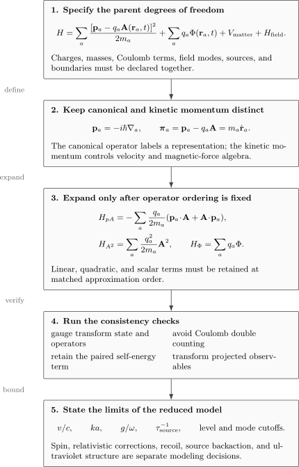
Minimal coupling is a linked ledger. The momentum definition, Hamiltonian expansion, gauge transformation, Coulomb bookkeeping, and approximation tests must be changed consistently.

Canonical Momentum and Kinetic Momentum

The distinction between canonical and kinetic momentum is already present in classical mechanics. For one charge in prescribed potentials, take

$$L = \frac{1}{2}m\dot{\mathbf r}^{\,2} + q\dot{\mathbf r}\mathbin{\cdot}\mathbf A(\mathbf r,t) - q\Phi(\mathbf r,t).$$

The canonical momentum is

$$\mathbf p \equiv \frac{\partial L}{\partial\dot{\mathbf r}} = m\dot{\mathbf r} + q\mathbf A.$$

The kinetic, mechanical, or gauge-covariant momentum is

$$\boldsymbol\pi \equiv m\dot{\mathbf r} = \mathbf p-q\mathbf A.$$

The Legendre transform gives

$$H = \frac{\boldsymbol\pi^2}{2m} + q\Phi = \frac{ \left( \mathbf p-q\mathbf A \right)^2 }{2m} + q\Phi.$$

Quantization promotes the canonical variables to operators satisfying

$$[r_i,p_j] = i\hbar\delta_{ij}.$$

In the position representation,

$$\mathbf p=-i\hbar\boldsymbol\nabla, \qquad \boldsymbol\pi = -i\hbar\boldsymbol\nabla-q\mathbf A.$$

The canonical commutator with position survives:

$$[r_i,\pi_j] = i\hbar\delta_{ij},$$

but kinetic-momentum components detect the magnetic field:

$$[\pi_i,\pi_j] = i\hbar q \sum_k \epsilon_{ijk}B_k.$$

Thus $\mathbf p$ supplies canonical translation generators in the chosen representation, whereas $\boldsymbol\pi$ supplies mechanical velocity and magnetic-force algebra. They agree only when the relevant vector potential vanishes in that representation.

Velocity and the Lorentz-force check

For

$$H = \frac{\boldsymbol\pi^2}{2m} + q\Phi + V(\mathbf r),$$

the Heisenberg velocity is

$$\dot{\mathbf r} = \frac{i}{\hbar}[H,\mathbf r] = \frac{\boldsymbol\pi}{m}.$$

The equation for kinetic momentum has the Hermitian Lorentz-force form

$$\begin{aligned} m\dot{\mathbf v} ={}& q\mathbf E \\ &+ \frac{q}{2} \left( \mathbf v\times\mathbf B - \mathbf B\times\mathbf v \right) - \boldsymbol\nabla V. \end{aligned}$$

When $\mathbf B$ commutes with $\mathbf v$, the magnetic term reduces to $q\mathbf v\times\mathbf B$. Recovering this equation is a useful sign and ordering check.

Gauge dependence and physical momentum

Under a gauge transformation,

$$\begin{aligned} \mathbf A' &= \mathbf A+\boldsymbol\nabla\chi, \\ \Phi' &= \Phi-\partial_t\chi, \\ \psi' &= e^{iq\chi/\hbar}\psi. \end{aligned}$$

The canonical differential operator $-i\hbar\boldsymbol\nabla$ has the same written form but acts on a differently phased wavefunction. The kinetic momentum transforms covariantly:

$$\boldsymbol\pi'\psi' = e^{iq\chi/\hbar} \boldsymbol\pi\psi.$$

Expectation values of mechanical momentum therefore agree when states and operators are transformed together. A bare canonical-momentum label in one gauge is not automatically a gauge-independent observable.

The Replacement p → p − qA

The rule

$$\mathbf p \longrightarrow \mathbf p-q\mathbf A$$

is best read inside the complete Hamiltonian. It does not mean that every occurrence of a momentum symbol in an already reduced model can be shifted without revisiting how that model was derived.

For one particle,

$$\begin{aligned} \frac{ \left( \mathbf p-q\mathbf A \right)^2 }{2m} ={}& \frac{\mathbf p^2}{2m} \\ &- \frac{q}{2m} \left( \mathbf p\mathbin{\cdot}\mathbf A + \mathbf A\mathbin{\cdot}\mathbf p \right) \\ &+ \frac{q^2\mathbf A^2}{2m}. \end{aligned}$$

The symmetrized cross term is required because $\mathbf p$ differentiates the position dependence of $\mathbf A$.

Acting on a wavefunction,

$$\begin{aligned} \left( \mathbf p-q\mathbf A \right)^2\psi ={}& -\hbar^2\nabla^2\psi \\ &+ iq\hbar \left( \boldsymbol\nabla\mathbin{\cdot}\mathbf A \right)\psi \\ &+ 2iq\hbar\, \mathbf A\mathbin{\cdot}\boldsymbol\nabla\psi + q^2\mathbf A^2\psi. \end{aligned}$$

In Coulomb gauge, $\boldsymbol\nabla\cdot\mathbf A=0$. Subject also to the domain and boundary conditions that make the operators well defined,

$$\mathbf p\mathbin{\cdot}\mathbf A = \mathbf A\mathbin{\cdot}\mathbf p.$$

Only then may the linear term be abbreviated as

$$H_{pA} = - \frac{q}{m} \mathbf A\mathbin{\cdot}\mathbf p.$$

Keeping the anticommutator form until the gauge and mode functions are fixed prevents an assumption from being mistaken for an identity.

Sign conventions

The charge $q$ includes its sign. For an electron,

$$q=-e, \qquad e>0,$$

so

$$\boldsymbol\pi_{\mathrm e} = \mathbf p+e\mathbf A.$$

Writing both $q=-e$ and an additional hand-inserted minus sign is a common source of incorrect Zeeman and interaction terms.

Dimensional check

All three quantities

$$\mathbf p, \qquad q\mathbf A, \qquad \boldsymbol\pi$$

have dimensions of momentum. For a monochromatic plane wave with electric field amplitude $\mathcal E_0$ and angular frequency $\omega$,

$$\mathcal E_0 = \omega A_0$$

in a transverse gauge with vector-potential amplitude $A_0$. Thus

$$|q|A_0 = \frac{|q|\mathcal E_0}{\omega}$$

is the field-induced momentum scale to compare with matter momenta.

The Scalar Potential

The scalar-potential contribution is

$$H_\Phi = q\Phi(\mathbf r,t).$$

Its sign follows the charge. An electron in a positive electrostatic potential has potential energy $-e\Phi$, while a positive ion has $+|q|\Phi$.

The electric field is

$$\mathbf E = - \boldsymbol\nabla\Phi - \partial_t\mathbf A.$$

Separating “electric coupling” into a scalar-potential part and a vector-potential part is therefore gauge dependent. A static longitudinal field is often conveniently represented by $\Phi$. A propagating transverse wave in Coulomb gauge is often represented with $\Phi=0$ and $\mathbf E=-\partial_t\mathbf A$. The measured field is independent of that bookkeeping.

Constant offsets and time-dependent phases

Adding a spatially uniform function $C(t)$ to the scalar potential shifts the Hamiltonian by $qC(t)$. For a fixed charge sector, this changes the state by a common time-dependent phase:

$$\psi(t) \longrightarrow \exp \left[ - \frac{iq}{\hbar} \int^t C(t')\,dt' \right] \psi(t).$$

It does not change probabilities within that charge sector. Relative phases between sectors with different total charge require more careful bookkeeping, especially when the charge reference or external circuit is part of the experiment.

External scalar fields versus internal Coulomb energy

For several charges, distinguish an imposed scalar potential $\Phi_{\mathrm{ext}}$ from the mutual Coulomb interaction. In Coulomb-gauge nonrelativistic QED, the longitudinal electric field can be eliminated in favor of the instantaneous Coulomb energy

$$V_{\mathrm C} = \frac{1}{8\pi\epsilon_0} \sum_{a\ne b} \frac{q_aq_b} {|\mathbf r_a-\mathbf r_b|}.$$

The $a=b$ self-terms are excluded here. If $V_{\mathrm C}$ is already present, adding the same longitudinal interaction again through a dynamical scalar potential double counts it.

This distinction is especially important in molecular Hamiltonians, where electron–electron, electron–nuclear, and nuclear–nuclear Coulomb energies are usually already included in $V_{\mathrm{matter}}$.

The A² Term

Expanding minimal coupling organizes the Hamiltonian as

$$H = H_0 + H_{pA} + H_{A^2} + H_\Phi,$$

where

$$\begin{aligned} H_{pA} &= - \frac{q}{2m} \left( \mathbf p\mathbin{\cdot}\mathbf A + \mathbf A\mathbin{\cdot}\mathbf p \right), \\ H_{A^2} &= \frac{q^2}{2m}\mathbf A^2, \\ H_\Phi &= q\Phi. \end{aligned}$$

$H_{pA}$ is often called the paramagnetic or linear coupling. $H_{A^2}$ is often called the diamagnetic, seagull, or quadratic coupling. The names describe their role in a chosen representation; they do not make the individual terms gauge-invariant observables.

Why quadratic does not mean optional

If the field amplitude is counted as a small parameter $\lambda$, then

$$H_{pA}=O(\lambda), \qquad H_{A^2}=O(\lambda^2).$$

A second-order calculation contains both first-order perturbation theory in $H_{A^2}$ and second-order perturbation theory in $H_{pA}$. Dropping one while keeping the other generally gives an incomplete result at $O(\lambda^2)$.

The quadratic term contributes to:

• diamagnetic response;
• field-frequency and mode renormalization;
• two-photon and counter-rotating processes;
• cancellations constrained by oscillator-strength sum rules;
• boundedness and stability properties of effective models;
• gauge equivalence with representations in which its role is carried by a polarization self-energy term.

Whether a particular observable is insensitive to $H_{A^2}$ is a conclusion to derive, not an assumption to import.

Current-density form

Define the charge density

$$\rho(\mathbf r) = \sum_a q_a \delta(\mathbf r-\mathbf r_a)$$

and the canonical paramagnetic current density

$$\mathbf j_{\mathrm p}(\mathbf r) = \sum_a \frac{q_a}{2m_a} \left\{ \mathbf p_a, \delta(\mathbf r-\mathbf r_a) \right\}.$$

Then the linear interaction can be written

$$H_{pA} = - \int d^3r\, \mathbf j_{\mathrm p}(\mathbf r) \mathbin{\cdot} \mathbf A(\mathbf r).$$

The scalar interaction is

$$H_\Phi = \int d^3r\, \rho(\mathbf r)\Phi(\mathbf r),$$

and the quadratic term is

$$H_{A^2} = \frac{1}{2} \int d^3r\, K(\mathbf r)\mathbf A^2(\mathbf r),$$

with

$$K(\mathbf r) = \sum_a \frac{q_a^2}{m_a} \delta(\mathbf r-\mathbf r_a).$$

This form makes two facts visible. Charge neutrality can cancel the spatial integral of $\rho$, but it does not cancel $K$, because the latter contains $q_a^2$. Also, the physical current contains both paramagnetic and field-dependent diamagnetic pieces; the split depends on representation.

Prescribed and quantized fields

For a prescribed field, $\mathbf A^2$ is a function of space and time. If it is spatially uniform over a one-particle system, it may be proportional to the identity in the matter Hilbert space, although it still contributes a phase and can matter when comparing gauges or coupled sectors.

For a quantized field, $\mathbf A^2$ is an operator on the field Hilbert space. For one real mode,

$$\mathbf A(\mathbf r) = A_{\mathrm{zpf}}\, \boldsymbol\epsilon f(\mathbf r) \left( a+a^\dagger \right),$$

so

$$\begin{aligned} \mathbf A^2(\mathbf r) ={}& A_{\mathrm{zpf}}^2 f^2(\mathbf r) \\ &\times \left( a^2 + a^{\dagger 2} + 2a^\dagger a + 1 \right). \end{aligned}$$

The quadratic coupling therefore contains number-conserving, two-photon, and vacuum terms. Normal ordering can rearrange the written constant, but it does not justify deleting the physical contribution fixed by the parent Hamiltonian.

Many-Particle Hamiltonian

For nonrelativistic charges interacting with a prescribed electromagnetic background,

$$\begin{aligned} H ={}& \sum_a \frac{ \left[ \mathbf p_a - q_a\mathbf A(\mathbf r_a,t) \right]^2 }{2m_a} \\ &+ \sum_a q_a\Phi_{\mathrm{ext}}(\mathbf r_a,t) + V_{\mathrm{matter}}. \end{aligned}$$

For electrons and nuclei,

$$\begin{aligned} q_i&=-e, & m_i&=m_e, \\ q_A&=Z_Ae, & m_A&=M_A. \end{aligned}$$

$V_{\mathrm{matter}}$ normally includes all mutual Coulomb interactions and any additional effective terms used at the stated accuracy.

Quantized transverse radiation in Coulomb gauge

In a periodic quantization volume $\mathcal V$, the transverse vector potential may be expanded as

$$\begin{aligned} \mathbf A_\perp(\mathbf r) ={}& \sum_{\mathbf k,\lambda} \left( \frac{\hbar} {2\epsilon_0\omega_{\mathbf k}\mathcal V} \right)^{1/2} \boldsymbol\epsilon_{\mathbf k\lambda} \\ &\times \left( a_{\mathbf k\lambda} e^{i\mathbf k\cdot\mathbf r} + a_{\mathbf k\lambda}^\dagger e^{-i\mathbf k\cdot\mathbf r} \right), \end{aligned}$$

where

$$\mathbf k \mathbin{\cdot} \boldsymbol\epsilon_{\mathbf k\lambda} = 0.$$

The free-field Hamiltonian is

$$H_{\mathrm{EM}} = \sum_{\mathbf k,\lambda} \hbar\omega_{\mathbf k} \left( a_{\mathbf k\lambda}^\dagger a_{\mathbf k\lambda} + \frac{1}{2} \right).$$

A Coulomb-gauge many-particle Hamiltonian can then be organized as

$$\begin{aligned} H ={}& \sum_a \frac{ \left[ \mathbf p_a - q_a\mathbf A_\perp(\mathbf r_a) \right]^2 }{2m_a} \\ &+ V_{\mathrm C} + \sum_a q_a\Phi_{\mathrm{ext}}(\mathbf r_a,t) + H_{\mathrm{EM}}. \end{aligned}$$

The quantized transverse field and the longitudinal Coulomb interaction have different roles. The displayed split is tied to Coulomb gauge; another representation can redistribute interaction and self-energy terms while leaving observables unchanged in the untruncated theory.

Second-quantized matter

For species $s$ with field operators $\Psi_s(\mathbf r)$, charges $q_s$, and masses $m_s$, a schematic second-quantized form is

$$\boldsymbol\pi_s \equiv -i\hbar\boldsymbol\nabla - q_s\mathbf A.$$

Then

$$\begin{aligned} H_{\mathrm m} ={}& \sum_s \int d^3r\, \Psi_s^\dagger(\mathbf r) \frac{\boldsymbol\pi_s^2}{2m_s} \Psi_s(\mathbf r) \\ &+ \sum_s \int d^3r\, \Psi_s^\dagger(\mathbf r) q_s\Phi_{\mathrm{ext}} \Psi_s(\mathbf r) \\ &+ V_{\mathrm{int}}. \end{aligned}$$

$V_{\mathrm{int}}$ must state whether Coulomb, pseudopotential, effective core, or other interactions are included. Normal ordering and ultraviolet regularization also belong to the model specification when field operators are evaluated at coincident points.

Minimal coupling does not alter exchange statistics. It changes the one-body covariant derivative and the associated current while the bosonic or fermionic algebra remains as specified.

Center-of-mass and internal motion

Define total canonical momentum and total charge by

$$\mathbf P = \sum_a\mathbf p_a, \qquad Q = \sum_a q_a.$$

If the vector potential is effectively uniform across the composite system,

$$\sum_a\boldsymbol\pi_a = \mathbf P-Q\mathbf A.$$

For a neutral atom or molecule, $Q=0$, so the total kinetic momentum equals $\mathbf P$ in this particular long-wavelength expression. That does not mean the internal system decouples from the field. The linear interaction is

$$H_{pA} = - \mathbf A \mathbin{\cdot} \sum_a \frac{q_a}{m_a}\mathbf p_a,$$

which generally remains nonzero because the charge-to-mass ratios differ. The quadratic coefficient

$$\sum_a\frac{q_a^2}{2m_a}$$

also remains nonzero. Neutrality cancels total charge, not charge-weighted internal currents or squared-charge terms.

Separating center-of-mass and internal motion in a magnetic field can be subtle because vector potentials mix coordinates and canonical momenta. Pseudomomentum or magnetic-translation methods may be more natural than a naive free center-of-mass separation.

Fixed nuclei are an approximation

In an electronic-structure calculation, nuclei are often held at fixed positions. Their kinetic minimal-coupling terms are then absent from the electronic Hamiltonian, but their charges still determine $V_{\mathrm{matter}}$, external-field energies, and the molecular dipole. Restoring nuclear motion is necessary for recoil, rotational and vibrational coupling, motional Stark effects, and momentum conservation.

The Born–Oppenheimer Scale Separation page owns the general electronic–nuclear approximation.

Classical and Quantized Field Models

The same minimal-coupling symbol can represent physically different models.

Field treatment	$\mathbf A,\Phi$	Energy exchange	What is omitted
prescribed classical background	specified functions	external source supplies or absorbs energy	source depletion, field fluctuations, matter–field entanglement
stochastic classical field	random functions with a stated law	average over source realizations	genuinely quantum field statistics
selected quantized modes	field operators	reversible exchange with retained modes	discarded continuum unless added as a reservoir
full or effective continuum	operator-valued mode expansion	emission, absorption, and propagation	ultraviolet and material response still require a model

Prescribed fields

If $\mathbf A(\mathbf r,t)$ is imposed, the matter Hamiltonian is explicitly time dependent. Matter energy need not be conserved:

$$\frac{d}{dt} \langle H_{\mathrm m}(t)\rangle = \left\langle \frac{\partial H_{\mathrm m}}{\partial t} \right\rangle$$

for unitary matter evolution. The missing energy is exchanged with the unmodeled source.

A laser pulse described this way can have a perfectly controlled phase and envelope. The approximation fails when source depletion, photon counting, vacuum fluctuations, or entanglement with the field controls the observable.

Quantized modes

When $\mathbf A$ is operator valued, the matter and field Hilbert spaces are combined:

$$\mathcal H = \mathcal H_{\mathrm m} \otimes \mathcal H_{\mathrm f}.$$

Minimal coupling can then exchange excitations, entangle matter with the field, shift mode frequencies, and create virtual dressing. A few-mode truncation must be justified by mode spacing, bandwidth, geometry, and the observable. A single lossless mode does not by itself produce irreversible spontaneous decay.

For a bright coherent state, replacing a retained mode operator by its coherent amplitude may recover a classical drive for suitable observables. This is a state- and observable-dependent limit, not an identity between classical and quantum fields.

Relation to Gauge Invariance

For many particles, define

$$U_\chi(t) = \exp \left[ \frac{i}{\hbar} \sum_a q_a\chi(\mathbf r_a,t) \right].$$

Under

$$\begin{aligned} \mathbf A' &= \mathbf A+\boldsymbol\nabla\chi, \\ \Phi' &= \Phi-\partial_t\chi, \\ |\Psi'\rangle &= U_\chi|\Psi\rangle, \end{aligned}$$

each kinetic momentum obeys

$$\boldsymbol\pi_a' = U_\chi \boldsymbol\pi_a U_\chi^\dagger.$$

For a time-dependent transformation, the Hamiltonian changes as

$$H' = U_\chi H U_\chi^\dagger + i\hbar \left( \partial_tU_\chi \right) U_\chi^\dagger.$$

The second term supplies the scalar-potential transformation. Transforming only $\mathbf A$, or only the state, produces a different model rather than a new representation of the same model.

What gauge transformations can redistribute

The following partitions need not be separately invariant:

Partition	Why it can change
canonical matter momentum versus field contribution	canonical variables depend on representation
$p\cdot A$ versus $A^2$ contributions	terms reorganize under unitary transformations
matter excitation versus photon excitation	subsystem definitions can be gauge dependent
instantaneous Coulomb versus polarization interaction	longitudinal and multipolar descriptions partition energy differently
bare versus interaction Hamiltonian	a representation can move terms across the split

The total predictions of a complete theory agree. Intermediate labels should not be given independent physical meaning unless they are tied to a gauge-invariant measurement protocol.

Approximation and transformation need not commute

Let $P$ project matter onto a finite set of levels and $U$ denote a unitary change of representation. In general,

$$PUP$$

is not unitary on the truncated subspace. Consequently,

$$P \left( UHU^\dagger \right) P$$

need not be unitarily equivalent to transforming the already projected Hamiltonian $PHP$.

This issue is weak when discarded levels and modes contribute negligibly at the requested accuracy. It becomes important in ultrastrong coupling, severe few-level truncations, and incomplete mode spaces. The modern literature contains several technically distinct prescriptions for constructing gauge-consistent effective models. The settled practical lesson is modest:

1. state the parent Hamiltonian and representation;
2. project states and observables consistently;
3. retain the self-energy term paired with the chosen representation;
4. test convergence in matter levels and field modes;
5. compare gauge-related formulations only at matched approximation order.

The detailed comparison of Coulomb, velocity, length, and multipolar representations belongs to Gauge Choices in Light–Matter Physics, not to a deletion of $A^2$ from the parent theory.

Worked Examples

A prescribed transverse plane wave

Take

$$\begin{aligned} \mathbf A(\mathbf r,t) ={}& A_0\boldsymbol\epsilon \cos \left( \mathbf k\mathbin{\cdot}\mathbf r-\omega t \right), \\ &\Phi=0. \end{aligned}$$

with

$$\mathbf k\mathbin{\cdot}\boldsymbol\epsilon=0.$$

The electric-field amplitude and cycle-averaged intensity are

$$\mathcal E_0=\omega A_0, \qquad I = \frac{1}{2} c\epsilon_0\mathcal E_0^2.$$

For a region where the mode is smooth and the stated transverse-gauge conditions apply,

$$H_{pA} = - \frac{q}{m} \mathbf A\mathbin{\cdot}\mathbf p, \qquad H_{A^2} = \frac{q^2\mathbf A^2}{2m}.$$

For a matter momentum scale $p$, the characteristic ratio is

$$\frac{U_{A^2}}{U_{pA}} \sim \frac{|q|A_0}{2p}.$$

Writing

$$v_{\mathrm q} \equiv \frac{|q|A_0}{m}, \qquad v\equiv\frac{p}{m},$$

gives

$$\frac{U_{A^2}}{U_{pA}} \sim \frac{v_{\mathrm q}}{2v}.$$

This is only a scale estimate. If a linear-coupling matrix element vanishes by symmetry, comparing typical amplitudes can miss the leading allowed process.

An electron in a uniform magnetic field

For an electron, $q=-e$, choose symmetric gauge

$$\mathbf A = \frac{1}{2} \mathbf B\times\mathbf r, \qquad \Phi=0.$$

Because $\boldsymbol\nabla\cdot\mathbf A=0$,

$$\begin{aligned} H ={}& \frac{\mathbf p^2}{2m_e} + \frac{e}{m_e} \mathbf A\mathbin{\cdot}\mathbf p \\ &+ \frac{e^2\mathbf A^2}{2m_e}. \end{aligned}$$

Using

$$\mathbf A\mathbin{\cdot}\mathbf p = \frac{1}{2} \mathbf B\mathbin{\cdot}\mathbf L,$$

one obtains

$$\begin{aligned} H ={}& \frac{\mathbf p^2}{2m_e} + \frac{e}{2m_e} \mathbf B\mathbin{\cdot}\mathbf L \\ &+ \frac{e^2}{8m_e} \left| \mathbf B\times\mathbf r \right|^2. \end{aligned}$$

The second term is the orbital Zeeman coupling and the third is the diamagnetic term. For weak fields in a nondegenerate bound state, their leading perturbative orders differ, but both descend from the same square. Orbital Magnetic Moments and Landau Levels own the corresponding physical applications.

One quantized cavity mode

For one charge and one real mode, let

$$\mathbf A(\mathbf r) = A_{\mathrm{zpf}} \boldsymbol\epsilon f(\mathbf r) \left( a+a^\dagger \right).$$

The linear term is

$$\begin{aligned} H_{pA} ={}& - \frac{qA_{\mathrm{zpf}}}{2m} \left( a+a^\dagger \right) \\ &\times \left\{ \boldsymbol\epsilon\mathbin{\cdot}\mathbf p, f(\mathbf r) \right\}, \end{aligned}$$

while

$$\begin{aligned} H_{A^2} ={}& \frac{q^2A_{\mathrm{zpf}}^2}{2m} f^2(\mathbf r) \\ &\times \left( a+a^\dagger \right)^2. \end{aligned}$$

If $f(\mathbf r)$ is replaced by a constant in the long-wavelength limit, the matter and field factors simplify. That replacement is independent of the decision to truncate the matter spectrum or apply a rotating-wave approximation.

A neutral composite system

For a spatially uniform vector potential, a neutral system has

$$\sum_a q_a=0$$

but

$$\sum_a \frac{q_a}{m_a}\mathbf p_a \ne \mathbf 0$$

in general. For a hydrogenic atom,

$$\begin{aligned} \sum_a \frac{q_a}{m_a}\mathbf p_a ={}& - \frac{e}{m_e}\mathbf p_e \\ &+ \frac{e}{M_N}\mathbf P_N. \end{aligned}$$

After center-of-mass separation, this becomes an internal relative-momentum coupling with a reduced-mass coefficient. Neutral atoms therefore interact with light even though their net charge vanishes. The later dipole approximation rewrites the leading internal coupling in terms of the electric dipole, rather than asserting that minimal coupling disappeared.

Limits of the Nonrelativistic Treatment

Minimal coupling is compatible with nonrelativistic quantum mechanics, but it does not make that theory exact.

Velocity and binding scales

The basic condition is

$$\frac{v}{c}\ll1.$$

For a hydrogenic bound state, a characteristic estimate is

$$\frac{v}{c} \sim \frac{Z\alpha}{n}.$$

Relativistic corrections become progressively more important as $Z\alpha$ increases or the requested precision resolves terms of order $(v/c)^2$ relative to the leading energy.

Spin and the Pauli Hamiltonian

Scalar minimal coupling describes orbital motion. For spin-$1/2$ matter, add magnetic-moment coupling:

$$H_{\mathrm P} = \frac{\boldsymbol\pi^2}{2m} + q\Phi - \boldsymbol\mu\mathbin{\cdot}\mathbf B,$$

where

$$\boldsymbol\mu = g\frac{q}{2m}\mathbf S$$

in the stated $g$-factor convention. The Pauli Hamiltonian card records the $g=2$ form.

Spin–orbit, Darwin, relativistic kinetic, anomalous-moment, and radiative terms arise from a more complete theory or its effective expansion. They should not be attributed to the scalar replacement $\mathbf p\to\mathbf p-q\mathbf A$ alone.

Pair creation and radiation

Nonrelativistic fixed-particle-number mechanics cannot describe:

• pair creation or annihilation;
• fully relativistic recoil;
• dynamical antiparticles;
• high-energy Compton processes;
• radiation reaction as a self-consistent relativistic field process.

Quantizing selected electromagnetic modes permits emission and absorption within a nonrelativistic matter model, but ultraviolet self-energy and high-frequency behavior still require regularization, renormalization, or a physically justified effective cutoff.

Model-regime ledger

Approximation	Control question	Typical failure
nonrelativistic matter	are $v/c$ and $Z\alpha$ small at the required accuracy?	fine structure, pair processes, relativistic recoil
prescribed field	is source depletion or field backaction negligible?	photon statistics, spontaneous emission, matter–field entanglement
fixed nuclei	are recoil and nuclear motion unresolved?	rovibrational coupling, recoil, motional effects
long wavelength	is $ka\ll1$ for the relevant state support?	multipoles, spatial gradients, recoil phase
few matter levels	are discarded levels far detuned and weakly coupled?	leakage, sum-rule violation, gauge dependence
few field modes	does the retained mode set cover the bandwidth and geometry?	irreversible decay, propagation, causality, mode renormalization
weak-field deletion of $A^2$	is the observable computed only to an order where its contribution is demonstrably absent?	incomplete second-order response, instability, gauge mismatch
point-particle coupling	is structure below the cutoff irrelevant?	ultraviolet sensitivity, finite-size and form-factor effects

Each row answers a different question. Passing one does not validate the others.

A Practical Construction Workflow

For an AMO minimal-coupling model:

1. list all charged species, masses, coordinates, and charge signs;
2. choose whether fields are prescribed, stochastic, selected quantum modes, or a continuum;
3. state the gauge and boundary conditions used to define the potentials;
4. specify whether mutual Coulomb interactions are already in $V_{\mathrm{matter}}$;
5. keep the covariant square intact until operator ordering is controlled;
6. identify $H_{pA}$, $H_{A^2}$, and $H_\Phi$ at a matched perturbative order;
7. separate center-of-mass and internal variables only after checking field variation across the system;
8. add spin and relativistic effective terms required by the target precision;
9. project matter levels and field modes together with the observables;
10. test convergence, gauge consistency, and limiting cases.

A reproducible calculation should record the resulting approximation chain, not only the final few-level Hamiltonian.

Common Mistakes

• Confusing canonical and kinetic momentum. The velocity is $\boldsymbol\pi/m$, not generally $\mathbf p/m$.
• Forgetting that $\mathbf p$ differentiates $\mathbf A$. The cross term is an anticommutator before additional conditions are imposed.
• Using the electron charge twice. Set $q=-e$ once and carry that sign through the formulas.
• Dropping $A^2$ because it is quadratic. It contributes at the same order as second-order perturbation theory in $p\cdot A$.
• Double counting the longitudinal Coulomb field. Do not include the same interaction in both $V_{\mathrm C}$ and an independent scalar-field degree of freedom.
• Assuming neutrality removes light coupling. Internal currents and squared-charge terms remain.
• Treating a prescribed laser as a quantized reservoir. A classical drive does not create vacuum fluctuations or spontaneous emission.
• Changing gauge after truncating without transforming the projection and observables.
• Equating a few-mode Hamiltonian with full electromagnetic QED.
• Assuming scalar minimal coupling contains spin, Darwin, spin–orbit, or anomalous-moment terms.
• Comparing gauge-dependent bare photon or matter occupations as if their subsystem definitions were universal.
• Using $p\cdot A$ and $-\mathbf d\cdot\mathbf E$ simultaneously without deriving a non-double-counting hybrid representation.

Exercises

1. Legendre transform for one charge

Starting from

$$L = \frac{1}{2}m\dot{\mathbf r}^{\,2} + q\dot{\mathbf r}\mathbin{\cdot}\mathbf A - q\Phi,$$

derive the canonical momentum and Hamiltonian.

Solution

The canonical momentum is

$$\mathbf p = \frac{\partial L}{\partial\dot{\mathbf r}} = m\dot{\mathbf r}+q\mathbf A.$$

Hence

$$\dot{\mathbf r} = \frac{\mathbf p-q\mathbf A}{m}.$$

The Legendre transform gives

$$H = \mathbf p\mathbin{\cdot}\dot{\mathbf r} - L.$$

Substitute $\mathbf p=m\dot{\mathbf r}+q\mathbf A$:

$$\begin{aligned} H ={}& \left( m\dot{\mathbf r}+q\mathbf A \right) \mathbin{\cdot}\dot{\mathbf r} \\ &- \left[ \frac{1}{2}m\dot{\mathbf r}^{\,2} + q\dot{\mathbf r}\mathbin{\cdot}\mathbf A - q\Phi \right] \\ ={}& \frac{1}{2}m\dot{\mathbf r}^{\,2} + q\Phi. \end{aligned}$$

Finally,

$$H = \frac{ \left( \mathbf p-q\mathbf A \right)^2 }{2m} + q\Phi.$$

2. Operator ordering

Show that

$$\left( \mathbf p-q\mathbf A \right)^2$$

acting on $\psi$ contains a term proportional to $\boldsymbol\nabla\cdot\mathbf A$. Under what condition does the cross term reduce to $-2q\mathbf A\cdot\mathbf p$?

Solution

Expand without commuting the factors:

$$\begin{aligned} \left( \mathbf p-q\mathbf A \right)^2 ={}& \mathbf p^2 \\ &- q \left( \mathbf p\mathbin{\cdot}\mathbf A + \mathbf A\mathbin{\cdot}\mathbf p \right) \\ &+ q^2\mathbf A^2. \end{aligned}$$

Since $\mathbf p=-i\hbar\boldsymbol\nabla$,

$$\begin{aligned} \mathbf p\mathbin{\cdot} \left( \mathbf A\psi \right) ={}& -i\hbar \left( \boldsymbol\nabla\mathbin{\cdot}\mathbf A \right)\psi \\ &- i\hbar \mathbf A\mathbin{\cdot}\boldsymbol\nabla\psi, \end{aligned}$$

whereas

$$\mathbf A\mathbin{\cdot}\mathbf p\psi = -i\hbar \mathbf A\mathbin{\cdot}\boldsymbol\nabla\psi.$$

Define

$$\mathcal K \equiv \left( \mathbf p-q\mathbf A \right)^2.$$

Then

$$\begin{aligned} \mathcal K\psi ={}& -\hbar^2\nabla^2\psi \\ &+ iq\hbar \left( \boldsymbol\nabla\mathbin{\cdot}\mathbf A \right)\psi \\ &+ 2iq\hbar \mathbf A\mathbin{\cdot}\boldsymbol\nabla\psi + q^2\mathbf A^2\psi. \end{aligned}$$

If $\boldsymbol\nabla\cdot\mathbf A=0$ and the common operator domain and boundary conditions introduce no extra terms, then

$$\mathbf p\mathbin{\cdot}\mathbf A = \mathbf A\mathbin{\cdot}\mathbf p,$$

and the cross term becomes $-2q\mathbf A\cdot\mathbf p$.

3. Many-particle gauge covariance

For

$$U_\chi = \exp \left[ \frac{i}{\hbar} \sum_a q_a\chi(\mathbf r_a,t) \right],$$

show that the kinetic momentum of particle $a$ transforms covariantly.

Solution

Let

$$\Psi'=U_\chi\Psi, \qquad \mathbf A' = \mathbf A+\boldsymbol\nabla\chi.$$

Write

$$\boldsymbol\pi_a' \equiv \mathbf p_a-q_a\mathbf A'.$$

Only the $a$th phase factor is differentiated by $\mathbf p_a$:

$$\mathbf p_aU_\chi\Psi = U_\chi \left[ \mathbf p_a + q_a\boldsymbol\nabla_a\chi \right]\Psi.$$

Therefore

$$\begin{aligned} \boldsymbol\pi_a'\Psi' ={}& U_\chi \left[ \begin{gathered} \mathbf p_a + q_a\boldsymbol\nabla_a\chi \\ - q_a\mathbf A - q_a\boldsymbol\nabla_a\chi \end{gathered} \right]\Psi \\ ={}& U_\chi\boldsymbol\pi_a\Psi. \end{aligned}$$

Thus

$$\boldsymbol\pi_a' = U_\chi\boldsymbol\pi_aU_\chi^\dagger.$$

4. Orbital and diamagnetic terms

For an electron in a uniform field $\mathbf B=B\hat{\mathbf z}$, use symmetric gauge to derive the orbital Zeeman and diamagnetic terms.

Solution

For $q=-e$,

$$H = \frac{ \left( \mathbf p+e\mathbf A \right)^2 }{2m_e},$$

and in symmetric gauge

$$\mathbf A = \frac{1}{2} \mathbf B\times\mathbf r.$$

Because $\boldsymbol\nabla\cdot\mathbf A=0$,

$$H = \frac{\mathbf p^2}{2m_e} + \frac{e}{m_e} \mathbf A\mathbin{\cdot}\mathbf p + \frac{e^2\mathbf A^2}{2m_e}.$$

The linear term is

$$\begin{aligned} \mathbf A\mathbin{\cdot}\mathbf p &= \frac{1}{2} \left( \mathbf B\times\mathbf r \right) \mathbin{\cdot}\mathbf p \\ &= \frac{1}{2} \mathbf B\mathbin{\cdot} \left( \mathbf r\times\mathbf p \right) \\ &= \frac{1}{2} \mathbf B\mathbin{\cdot}\mathbf L. \end{aligned}$$

Also,

$$\mathbf A^2 = \frac{B^2}{4} \left( x^2+y^2 \right).$$

Hence

$$H = \frac{\mathbf p^2}{2m_e} + \frac{eB}{2m_e}L_z + \frac{e^2B^2}{8m_e} \left( x^2+y^2 \right).$$

5. Neutrality does not cancel A²

Consider particles in a spatially uniform vector potential. Show that the total-charge cancellation for a neutral system does not cancel either the linear internal coupling or the quadratic term.

Solution

The expanded interaction is

$$\begin{aligned} H_{\mathrm{int}} ={}& - \mathbf A\mathbin{\cdot} \sum_a \frac{q_a}{m_a}\mathbf p_a \\ &+ \mathbf A^2 \sum_a \frac{q_a^2}{2m_a}, \end{aligned}$$

where the transverse-gauge commutation conditions have been used.

Neutrality states only

$$\sum_aq_a=0.$$

It does not imply

$$\sum_a \frac{q_a}{m_a}\mathbf p_a=0$$

because masses and momenta differ. It also cannot cancel

$$\sum_a\frac{q_a^2}{2m_a},$$

whose nonzero terms all have positive $q_a^2/m_a$. A neutral composite can therefore have both internal linear coupling and a quadratic coupling.

6. Photon-number dependence of A²

For one mode, compute

$$\langle n| \left( a+a^\dagger \right)^2 |n\rangle.$$

Identify which terms change photon number by two.

Solution

Expand:

$$\left( a+a^\dagger \right)^2 = a^2 + a^{\dagger2} + aa^\dagger + a^\dagger a.$$

Using

$$aa^\dagger = a^\dagger a+1,$$

gives

$$\left( a+a^\dagger \right)^2 = a^2 + a^{\dagger2} + 2a^\dagger a + 1.$$

The diagonal expectation is

$$\langle n| \left( a+a^\dagger \right)^2 |n\rangle = 2n+1.$$

$a^2$ lowers photon number by two and $a^{\dagger2}$ raises it by two. The $2a^\dagger a+1$ part is diagonal in the number basis.

7. Uniform scalar-potential shift

Suppose $\Phi'(\mathbf r,t)=\Phi(\mathbf r,t)+C(t)$ for one particle. Find a phase transformation that removes $C(t)$ from the Schrödinger equation.

Solution

The shifted Hamiltonian is

$$H'=H+qC(t).$$

Let

$$\psi'(t) = \exp \left[ - \frac{iq}{\hbar} \int_{t_0}^{t} C(t')\,dt' \right] \psi(t).$$

Call the exponential prefactor $f(t)$. It obeys

$$i\hbar\partial_t f(t) = qC(t)f(t).$$

Differentiating $\psi'=f\psi$ gives

$$i\hbar\partial_t\psi' = qC(t)\psi' + f(t) i\hbar\partial_t\psi.$$

If $i\hbar\partial_t\psi=H\psi$, then

$$i\hbar\partial_t\psi' = \left( H+qC(t) \right)\psi' = H'\psi'.$$

The shift changes only a common phase within the fixed-charge sector.

8. Relativistic validity estimate

Use $v/c\sim Z\alpha/n$ to estimate the characteristic speed for a hydrogenic $1s$ electron at $Z=1$, $Z=20$, and $Z=80$. Interpret the result without treating the estimate as a precision calculation.

Solution

For $n=1$ and $\alpha\simeq1/137$,

$$\frac{v}{c} \sim \frac{Z}{137}.$$

Therefore

$$\begin{array}{c|c} Z & v/c \\ \hline 1 & 0.0073 \\ 20 & 0.146 \\ 80 & 0.584 \end{array}$$

For hydrogen, the nonrelativistic hierarchy is strong. At $Z=20$, relativistic corrections are no longer negligible in precision structure calculations. At $Z=80$, the estimate is not small, so a relativistic description is essential. Screening, finite nuclear size, electron correlation, and the Dirac spectrum are needed for quantitative multi-electron predictions; the simple $Z\alpha$ estimate is only a regime diagnostic.

Further Connections

• Light–Matter Interaction Overview places this parent Hamiltonian in the larger model ladder.
• Minimal Coupling in Wave Mechanics derives the position-space equation and conserved current.
• Gauge Transformations in Quantum Mechanics owns gauge-equivalent states, operators, and observables.
• Dipole Approximation derives the controlled long-wavelength reduction of this parent Hamiltonian and separates internal from center-of-mass phase variation.
• Transition Rates in Light–Matter Interaction develops weak-coupling rates after the interaction is chosen.
• Multipole Operators organizes the electric and magnetic multipoles that emerge after a controlled spatial expansion.
• Charged Particle in a Magnetic Field supplies the compact Hamiltonian card.

References

• C. Cohen-Tannoudji, J. Dupont-Roc, and G. Grynberg, Photons and Atoms: Introduction to Quantum Electrodynamics, Wiley, 1989.
• D. P. Craig and T. Thirunamachandran, Molecular Quantum Electrodynamics, Dover, 1998.
• R. G. Woolley, “Molecular quantum electrodynamics,” Proceedings of the Royal Society A 321, 557–572 (1971), doi:10.1098/rspa.1971.0049.
• E. A. Power and S. Zienau, “Coulomb gauge in non-relativistic quantum electro-dynamics and the shape of spectral lines,” Philosophical Transactions of the Royal Society A 251, 427–454 (1959), doi:10.1098/rsta.1959.0008.
• M. Babiker and R. Loudon, “Derivation of the Power–Zienau–Woolley Hamiltonian in quantum electrodynamics by gauge transformation,” Proceedings of the Royal Society A 385, 439–460 (1983), doi:10.1098/rspa.1983.0022.
• K. Rzażewski, K. Wódkiewicz, and W. Żakowicz, “Phase transitions, two-level atoms, and the $A^2$ term,” Physical Review Letters 35, 432–434 (1975), doi:10.1103/PhysRevLett.35.432.
• A. Stokes and A. Nazir, “Gauge ambiguities imply Jaynes–Cummings physics remains valid in ultrastrong coupling QED,” Nature Communications 10, 499 (2019), doi:10.1038/s41467-018-08101-0.
• O. Di Stefano et al., “Resolution of gauge ambiguities in ultrastrong-coupling cavity quantum electrodynamics,” Nature Physics 15, 803–808 (2019), doi:10.1038/s41567-019-0534-4.
• A. Stokes and A. Nazir, “Implications of gauge freedom for nonrelativistic quantum electrodynamics,” Nature Physics 20, 376–378 (2024), doi:10.1038/s41567-023-02155-8.
• O. Di Stefano et al., “Reply to: Implications of gauge freedom for nonrelativistic quantum electrodynamics,” Nature Physics 20, 379–380 (2024), doi:10.1038/s41567-023-02178-1.
• A. Vukics, G. Kónya, and P. Domokos, “The gauge-invariant Lagrangian, the Power–Zienau–Woolley picture, and the choices of field momenta in nonrelativistic quantum electrodynamics,” Scientific Reports 11, 16337 (2021), doi:10.1038/s41598-021-94405-z.
• C. Gustin, S. Franke, and S. Hughes, “Gauge-invariant theory of truncated quantum light–matter interactions in arbitrary media,” Physical Review A 107, 013722 (2023), doi:10.1103/PhysRevA.107.013722.