Rabi Oscillations

Rabi oscillations are coherent, reversible oscillations of population between two driven quantum states. They occur when a phase-stable field couples the states strongly enough that amplitude transferred into the second state can return before relaxation, dephasing, leakage, or ensemble averaging erases the phase relation.

For a constant drive, an atom prepared in $|g\rangle$, and the convention

$$H_{\mathrm{RWA}} = \frac{\hbar}{2} \left( \Delta\sigma_z+\Omega\sigma_\phi \right),$$

the ideal excited-state probability is

$$\begin{aligned} P_e(t) &= \frac{\Omega^2}{\Omega_R^2} \sin^2\!\left( \frac{\Omega_Rt}{2} \right), \\ \Omega_R &= \sqrt{\Omega^2+\Delta^2}. \end{aligned}$$

This compact trace contains several experimentally distinct quantities: oscillation frequency, amplitude, phase, offset, and envelope. Treating all of them as “the Rabi frequency” hides useful diagnostics.

Canonical Scope

Rabi Oscillations: First Encounter owns the closed-system derivation of the formula above. This page uses that result as an AMO diagnostic and control tool. It owns:

1. mapping a physical transition matrix element and field amplitude to $\Omega$;
2. interpreting resonant and detuned population traces;
3. defining $\pi$, $\pi/2$, and general pulse areas with their assumptions;
4. reading a two-dimensional Rabi chevron;
5. separating oscillation frequency, contrast, offset, and damping;
6. identifying multilevel, motional, readout, and open-system failure signatures.

Other canonical handoffs are equally important:

• Two-Level Atom owns the multilevel projection, frame convention, and detuning sign.
• Resonant Driving owns finite-time Fourier width and the bridge from first-order secular growth to exact two-state dynamics.
• Rotating-Wave Approximation owns the error analysis for discarded counter-rotating terms.
• Rabi and Ramsey Control owns protocol-level calibration under relaxation, dephasing, and control error.
• Ramsey Interferometry owns the AMO separated-pulse unitary, fringes, detuning estimators, and atomic-clock discriminator.
• Time-Dependent Two-Level Systems Notebook owns executable detuned Rabi traces, full laboratory-frame versus RWA propagation, equal-area pulse-shape tests, and finite-pulse Ramsey benchmarks.
• Optical Bloch Equations owns the AMO damping, steady-state, saturation, and fluorescence dictionary. The open-system treatment owns the general Markovian derivation.

Resonant Rabi Oscillations

Population exchange

On exact effective resonance,

$$\Delta_{\mathrm{eff}} = 0,$$

and a square pulse gives

$$P_e(t) = \sin^2\!\left( \frac{\Omega t}{2} \right).$$

Starting in $|g\rangle$, the state is

$$\begin{aligned} |\psi(t)\rangle ={}& \cos\!\left( \frac{\Omega t}{2} \right)|g\rangle \\ &- i e^{-i\phi} \sin\!\left( \frac{\Omega t}{2} \right)|e\rangle. \end{aligned}$$

The drive phase $\phi$ does not change the population in this single-pulse, ground-state experiment, but it does set the phase of the created coherence. It becomes observable when another pulse, another coupling path, or state tomography supplies a phase reference.

Oscillation period

Because $P_e$ contains $\sin^2(\Omega t/2)$, its period is

$$T_R = \frac{2\pi}{\Omega}.$$

The state vector changes sign after one full population period:

$$|\psi(T_R)\rangle = -|g\rangle.$$

That minus sign is a global phase for this isolated sequence. It can become relative phase if the driven subspace is embedded in a larger coherent Hilbert space.

Coherent oscillation is not a transition rate

Fermi’s golden rule describes approximately irreversible transfer into a continuum or dense set of final states over an appropriate time window. A closed resonant pair instead exchanges amplitude coherently. The population can return because the drive preserves phase and the final state is not a continuum sink.

The two pictures connect in different limits but should not be combined by inserting a golden-rule rate into the sinusoid. Transition Rates in Light–Matter Interaction owns the rate dictionary.

What the detector actually sees

State preparation and measurement need not map $P_e=0$ to a zero signal or $P_e=1$ to a unit signal. If the mean readouts for known ground and excited states are $S_g$ and $S_e$, an ideal linear detector gives

$$S(t) = S_g + \left( S_e-S_g \right) P_e(t).$$

Equivalently, a normalized but imperfect binary classifier may report

$$P_{\mathrm{obs}}(t) = p_{e|g} + \left( p_{e|e}-p_{e|g} \right) P_e(t),$$

where $p_{e|g}$ is the false-positive probability and $p_{e|e}$ is the true-positive probability. Readout error changes offset and contrast; it does not by itself change the coherent oscillation frequency.

Phase-coherent evidence

A reproducible oscillatory trace is evidence that preparation, drive, and readout retain phase information over several cycles. It is not, by itself, a complete characterization of coherence. Classical amplitude modulation, readout transients, multiple unresolved frequencies, or postselection can distort or imitate portions of a trace. Phase shifts, tomography, power scaling, and model enlargement provide stronger checks.

Detuned Rabi Oscillations

Tilted rotation axis

For constant detuning,

$$\boldsymbol\Omega_{\mathrm{eff}} = \left( \Omega\cos\phi, \Omega\sin\phi, \Delta \right).$$

The Bloch vector rotates around this tilted axis. Its angular speed is $\Omega_R$, but only the transverse component can move an initial $-\widehat{\mathbf z}$ vector toward the excited pole. Hence

$$P_e^{\mathrm{max}} = \frac{\Omega^2}{\Omega^2+\Delta^2}.$$

Detuning therefore causes two simultaneous changes:

1. the oscillation frequency increases from $\Omega$ to $\Omega_R$;
2. the maximum transfer decreases below unity.

A faster oscillation does not imply a stronger resonant coupling.

Inferring coupling and detuning

If an ideal trace determines both $\Omega_R$ and its maximum $A$, then

$$\begin{aligned} |\Omega| &= \Omega_R\sqrt A, \\ |\Delta| &= \Omega_R\sqrt{1-A}. \end{aligned}$$

The sign of detuning is absent from a population trace because the ideal formula contains $\Delta^2$. It must be obtained from a frequency reference, a phase-sensitive measurement, a known scan direction, or an asymmetric shift.

Unknown readout contrast breaks this simple inversion. A reduced measured amplitude can be caused by detuning, readout error, state-preparation error, leakage, damping, or ensemble inhomogeneity.

Effective resonance center

The detuning in the trace is the complete rotating-frame detuning,

$$\Delta_{\mathrm{eff}} = \omega_0 + \delta\omega_{\mathrm{shift}} - \omega_L.$$

The shift can depend on drive power. An ac Stark or Bloch–Siegert shift can move the center of a Rabi chevron as power changes. Fixing the center at the zero-power spectroscopic frequency can therefore bias the fitted $\Omega$.

The Rabi chevron

A Rabi chevron plots measured population versus pulse duration and drive frequency or detuning. In the ideal model,

$$P_e(t,\Delta) = \frac{\Omega^2}{\Omega^2+\Delta^2} \sin^2\!\left[ \frac{t}{2} \sqrt{\Omega^2+\Delta^2} \right].$$

The central resonant column reaches the largest contrast. Away from resonance, the oscillations become faster and shallower, producing curved fringes. A two-dimensional fit separates $\Omega$, resonance center, and readout contrast more reliably than one trace if the model is correct.

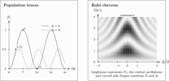
Left: a resonant trace reaches unit population, while the example $\Delta=\Omega$ trace oscillates at $\sqrt2\,\Omega$ with maximum $1/2$. Right: an ideal Rabi chevron encodes coupling, resonance center, and contrast in a two-dimensional pattern. Real data add offsets, damping, inhomogeneity, leakage, and power-dependent shifts.

What asymmetry means

The ideal square-pulse chevron is even in $\Delta$. Left–right asymmetry can signal:

• a power-dependent resonance shift correlated with pulse amplitude;
• frequency-dependent delivery or detector response;
• interference with a second transition;
• chirp during the pulse;
• asymmetric pulse-spectrum side lobes;
• a scan axis that is not the true detuning.

Asymmetry is information. Symmetrizing the data before diagnosing it can erase the mechanism.

Ensemble averaging

If atoms experience a distribution $f(\Delta)$, the observed population is

$$\overline{P_e}(t) = \int d\Delta\, f(\Delta) P_e(t,\Delta).$$

The average can show a decaying envelope even if every atom evolves unitarily. Spatial intensity variation similarly averages over a distribution of $\Omega$. A damped trace therefore does not uniquely identify irreversible decoherence.

Rabi Frequency

Convention-independent definition

Write the near-resonant part of a Hermitian interaction as

$$\begin{aligned} V(t) &= V^{(+)}e^{-i\omega_Lt} + V^{(-)}e^{i\omega_Lt}, \\ V^{(-)} &= \left( V^{(+)} \right)^\dagger. \end{aligned}$$

The complex Rabi amplitude is

$$\Omega_c \equiv \frac{2}{\hbar} \langle e|V^{(+)}|g\rangle.$$

Its magnitude $\Omega=|\Omega_c|$ sets the resonant population period, and its phase sets the equatorial control axis. This definition exposes the factor of two: $V^{(+)}$ is one complex-frequency component of a real oscillating field.

Electric-dipole coupling

For

$$\mathbf E(t) = \mathcal E_0 \widehat{\boldsymbol\epsilon} \cos(\omega_Lt+\phi),$$

the positive-frequency interaction can be written

$$V^{(+)} = - \frac{\mathcal E_0}{2} e^{-i\phi} \mathbf d\mathbin{\cdot} \widehat{\boldsymbol\epsilon}.$$

Therefore

$$\Omega_c = - \frac{\mathcal E_0}{\hbar} e^{-i\phi} \langle e| \mathbf d\mathbin{\cdot} \widehat{\boldsymbol\epsilon} |g\rangle.$$

For a plane wave in vacuum,

$$I = \frac12c\epsilon_0\mathcal E_0^2,$$

so an unsaturated E1 coupling obeys

$$\Omega \propto \mathcal E_0 \propto \sqrt I.$$

At fixed beam profile, $I\propto P$ and hence $\Omega\propto\sqrt P$. This square-root scaling is a useful calibration check, not a universal law under arbitrary power broadening, saturation of upstream optics, beam reshaping, or field-dependent state mixing.

Polarization and angular factors

In a spherical basis,

$$\Omega_c = - \frac{\mathcal E_0}{\hbar} e^{-i\phi} \sum_{q=-1}^{1} \epsilon_q \langle e|d_q|g\rangle.$$

The matrix element contains the reduced electronic or molecular strength and the angular coefficient for the selected magnetic sublevels. Polarization impurity can therefore create both a calibration error in the target $\Omega$ and leakage through unwanted $q$ components.

Dipole Transitions owns the Wigner–Eckart and polarization selection-rule derivation.

M1, E2, and effective couplings

The same operational definition applies beyond E1:

$$\Omega = \frac{2}{\hbar} \left| \langle e|V^{(+)}|g\rangle \right|.$$

For M1, $V^{(+)}$ contains the magnetic field and transition magnetic moment. For E2, it contains the electric-field gradient and transition quadrupole tensor. A Raman $\Omega$ contains products of one-photon couplings divided by an intermediate detuning, together with light shifts and scattering corrections.

Multipole Expansion owns the M1 and E2 operator conventions. Adiabatic Elimination owns effective Raman reductions.

Local field versus nominal power

The atom responds to the local mode amplitude, not the number displayed by a power meter. A calibration must account for:

• beam waist and position;
• standing-wave phase;
• polarization at the atom;
• window and fiber transmission;
• microwave impedance and near-field geometry;
• cavity enhancement;
• pulse-shape distortion and switching transients.

For a Gaussian beam, motion through the intensity profile creates a distribution of $\Omega$. In a standing wave, the same nominal power can give a node or antinode depending on position.

Frequency labels

Three frequencies should not be conflated:

• Bare transition frequency: $\omega_0$ before applied-field shifts.
• Rabi frequency: $\Omega$, the resonant transverse coupling in the stated convention.
• Generalized Rabi frequency: $\Omega_R=\sqrt{\Omega^2+\Delta^2}$, the rotation rate of the constant RWA Hamiltonian.

An observed oscillation frequency equals $\Omega_R$ in the ideal model, not automatically $\Omega$.

π and π/2 Pulses

Pulse area

On exact effective resonance with fixed drive phase,

$$H(t) = \frac{\hbar\Omega(t)}{2}\sigma_\phi.$$

Hamiltonians at different times commute because they are proportional to the same Pauli operator. The pulse is therefore characterized by its area

$$\Theta \equiv \int_{t_i}^{t_f} \Omega(t)\,dt.$$

For an initial ground state,

$$P_e = \sin^2\!\left( \frac{\Theta}{2} \right).$$

This area theorem is exact within the resonant two-level RWA model even for a shaped amplitude.

Named pulse areas

• A $\pi/2$ pulse has $\Theta=\pi/2$ and creates equal populations from an initial pole state.
• A $\pi$ pulse has $\Theta=\pi$ and inverts an initial pole state.
• A $2\pi$ pulse has $\Theta=2\pi$ and returns the population while the state vector acquires a minus sign.

For a square resonant pulse,

$$\begin{aligned} t_{\pi/2} &= \frac{\pi}{2\Omega}, \\ t_\pi &= \frac{\pi}{\Omega}, \\ t_{2\pi} &= \frac{2\pi}{\Omega}. \end{aligned}$$

A π/2 pulse is not a unique state

Starting from $|g\rangle$, a resonant $\pi/2$ pulse produces

$$|\psi_{\pi/2}\rangle = \frac{1}{\sqrt2} \left( |g\rangle - i e^{-i\phi}|e\rangle \right).$$

Changing $\phi$ moves the state around the equator. “Prepare a 50–50 superposition” is incomplete unless the relative phase is specified or irrelevant to the subsequent observable.

Amplitude error

Suppose a nominal $\pi$ pulse has a fractional area error $\epsilon$:

$$\Theta = \pi(1+\epsilon).$$

Then

$$\begin{aligned} P_e &= \sin^2\!\left[ \frac{\pi}{2}(1+\epsilon) \right] \\ &= \cos^2\!\left( \frac{\pi\epsilon}{2} \right) \\ &\simeq 1-\frac{\pi^2\epsilon^2}{4}. \end{aligned}$$

Population inversion is quadratically insensitive to a small area error at the top of the fringe. This does not mean the full unitary error is absent; phase and action on other input states can remain first order.

Detuning breaks the area-only rule

When $\Delta\ne0$,

$$H(t) = \frac{\hbar}{2} \left[ \Delta\sigma_z + \Omega(t)\sigma_\phi \right].$$

Changing $\Omega(t)$ changes the direction as well as the length of the effective field. Hamiltonians at different times need not commute, and $\int\Omega\,dt=\pi$ no longer guarantees inversion. Chirp, detuning, phase modulation, and pulse shaping require the time-ordered evolution or a justified effective construction.

Spatial and shot-to-shot area distributions

If different atoms or experimental shots experience different pulse areas, the average is

$$\overline{P_e} = \int d\Theta\, f(\Theta) \sin^2\!\left( \frac{\Theta}{2} \right).$$

This averaging reduces contrast even without irreversible decoherence. Composite and adiabatic pulses can trade duration, bandwidth, and sensitivity to make the transfer more robust, but they are not identical to a simple $\pi$ rotation.

Experimental Signatures

Prepare, drive, read

A time-domain Rabi experiment has three logically distinct stages:

1. prepare a known state or population distribution;
2. apply a phase-stable drive for a controlled duration;
3. measure the final state with calibrated errors.

Repeating the sequence for many pulse durations estimates the transition probability. Repeating each duration many times estimates statistical uncertainty.

What to extract from a trace

A useful trace report separates:

• fitted oscillation frequency;
• initial phase or timing offset;
• upper and lower signal levels;
• contrast;
• envelope shape and timescale;
• long-time baseline or steady value;
• residual structure;
• number of repetitions and statistical model.

An empirical fit such as

$$\begin{aligned} S(t) ={}& B + C \exp\!\left[ - \left( \frac{t}{T_R} \right)^\alpha \right] \\ &\times \cos(\Omega_{\mathrm{fit}}t+\varphi_0) \end{aligned}$$

can summarize a trace. It is not automatically a microscopic model. $\alpha=1$ may suggest an exponential Markovian envelope, while $\alpha=2$ may arise from quasi-static Gaussian inhomogeneity, but several mechanisms can produce similar forms over a limited range.

Binary readout statistics

For projective binary readout, if $k_j$ excited outcomes are observed in $N_j$ repetitions at pulse duration $t_j$, a natural likelihood is

$$k_j \sim \operatorname{Binomial} \left( N_j,p_j \right).$$

Fitting unweighted least squares to estimated probabilities assumes equal variance, whereas binomial variance

$$\operatorname{Var} \left( \frac{k_j}{N_j} \right) = \frac{ p_j(1-p_j) }{ N_j }$$

depends on population. Likelihood-based or appropriately weighted fits are preferable when precision matters.

Power scaling

For an E1 transition with unchanged mode and polarization,

$$\Omega \propto \sqrt P.$$

A plot of fitted resonant $\Omega$ versus $\sqrt P$ should be linear in the regime where the field delivery and two-level model are stable. Curvature can reveal:

• amplifier compression;
• power-meter or attenuator calibration error;
• changing beam waist or alignment;
• ac Stark shifts corrupting a fixed-frequency trace;
• multilevel dressing;
• a transition mechanism with different field dependence.

Chevron diagnostics

A good chevron fit should reproduce more than the central oscillation. It should also reproduce:

• curvature of the side fringes;
• contrast reduction with detuning;
• resonance-center motion with power;
• symmetry under detuning reversal when expected;
• pulse-start phase and timing offsets.

Structured residuals are often more informative than a small quoted uncertainty from an inadequate model.

Multiple frequencies

Beating or collapse and revival can indicate a distribution of coherent couplings rather than simple decoherence. Examples include:

• unresolved Zeeman or hyperfine transitions;
• motional-state-dependent sideband Rabi frequencies;
• spatially varying intensity;
• photon-number-dependent coupling to a quantized mode;
• coherent leakage into a third state.

A single damped sinusoid can hide these mechanisms.

Decoherence Effects

Markovian Bloch preview

Let

$$\mathbf r = (u,v,w), \qquad w = \rho_{ee}-\rho_{gg}.$$

For one common Markovian model,

$$\begin{aligned} \dot u &= -\Delta v-\Gamma_2u, \\ \dot v &= \Delta u-\Omega w-\Gamma_2v, \\ \dot w &= \Omega v-\Gamma_1(w-w_{\mathrm{eq}}). \end{aligned}$$

Here $\Gamma_1$ is the longitudinal population-relaxation rate, $\Gamma_2$ is the transverse coherence-decay rate, and $w_{\mathrm{eq}}$ is the equilibrium inversion. These equations assume a Markovian environment and the same rotating-frame/RWA conventions as the coherent model.

Resonant damping rate

On resonance, the homogeneous $(v,w)$ subsystem has eigenvalues

$$\lambda_\pm = - \frac{\Gamma_1+\Gamma_2}{2} \pm i \sqrt{ \Omega^2 - \frac{ (\Gamma_1-\Gamma_2)^2 }{ 4 } }.$$

When the drive is fast compared with the rates, the oscillatory envelope decays approximately at

$$\Gamma_R \simeq \frac{\Gamma_1+\Gamma_2}{2}.$$

For purely radiative decay with no additional pure dephasing,

$$\Gamma_2 = \frac{\Gamma_1}{2}, \qquad \Gamma_R \simeq \frac{3\Gamma_1}{4}.$$

This coefficient is model specific. It should not be fitted to data and then interpreted as universal when drive noise, detuning noise, inhomogeneity, leakage, or non-Markovian memory is appreciable.

Quasi-static amplitude noise

Suppose the resonant Rabi frequency varies between shots as

$$\Omega' = \Omega(1+\epsilon),$$

where $\epsilon$ is Gaussian with zero mean and standard deviation $\sigma_\epsilon$. Averaging the oscillatory cosine gives

$$\left\langle \cos(\Omega't) \right\rangle = \cos(\Omega t) \exp\!\left[ - \frac12 \left( \sigma_\epsilon\Omega t \right)^2 \right].$$

The envelope is Gaussian and decays faster at larger drive amplitude. That scaling distinguishes quasi-static fractional amplitude noise from a fixed Markovian relaxation rate.

Detuning noise

Quasi-static detuning noise averages traces with different $\Omega_R=\sqrt{\Omega^2+\Delta^2}$. Exactly at mean resonance, small detuning enters the oscillation frequency only to second order but still tilts the rotation axis and changes transfer amplitude. Away from resonance, the frequency is first-order sensitive to detuning fluctuations.

Ramsey experiments are usually more sensitive to low-frequency detuning noise because phase accumulates during a free-evolution interval. The separated-field sequence, fringes, and clock discriminator are developed in Ramsey Interferometry; the comparison with echo and other open-system controls belongs to Rabi and Ramsey Control.

Relaxation, dephasing, and leakage

These mechanisms leave different idealized signatures:

• Relaxation: changes the long-time population and damps oscillations.
• Pure dephasing: damps transverse coherence without direct population loss in the energy basis.
• Leakage: moves population outside the two-state normalization and may produce additional frequencies.
• Readout drift: changes apparent offset or contrast without changing the underlying state.
• Inhomogeneous averaging: produces reversible ensemble decay that may respond to echo or selection.

One trace rarely identifies all of them. Varying power, detuning, initial state, pulse phase, and delay supplies independent constraints.

Scope and Limitations

Square-pulse model

The closed formula assumes constant $\Omega$, $\Delta$, and $\phi$ during the pulse. Ringing, chirp, finite rise time, phase transients, and pulse distortion change the propagator. Replacing the programmed waveform by the field measured at the source may still miss distortion at the atom.

Two-level closure

Strong drive and broad pulses can excite spectator levels. A trace can remain oscillatory while the frequency and contrast are shifted by multilevel dressing. Check the leakage and virtual-shift ledger in Two-Level Atom.

Rotating-wave regime

When $\Omega$ is not small compared with $\omega_0+\omega_L$, counter-rotating dynamics changes the resonance and waveform. A fitted sinusoid can then return a convention-dependent effective frequency rather than the weak-drive Rabi frequency.

Quantized field

For a two-level emitter coupled to a quantized mode, different photon-number sectors have different oscillation frequencies. In the Jaynes–Cummings convention

$$H_{\mathrm{int}} = \hbar g \left( a\sigma_+ + a^\dagger\sigma_- \right),$$

the pair $|e,n\rangle$ and $|g,n+1\rangle$ oscillates at

$$\Omega_n = 2g\sqrt{n+1}.$$

A coherent field contains many $n$ values and can produce collapse and revival rather than one sinusoid. Jaynes–Cummings Model owns that quantized-mode model.

Evidence and inference

Rabi flopping is a strong coherence diagnostic, but a trustworthy claim also states:

• the preparation and measurement model;
• the range of pulse durations and powers;
• the number of visible cycles;
• the fit likelihood and residuals;
• alternative multilevel or classical explanations tested;
• the uncertainty and stability of $\Omega$ and resonance center.

A Practical Analysis Workflow

1. Calibrate the readout endpoints. Measure known $|g\rangle$ and $|e\rangle$ preparations when possible.
2. Locate resonance at low power. Minimize power-dependent shifts while identifying the target line.
3. Acquire a short Rabi trace. Estimate $\Omega_R$, timing offsets, and contrast.
4. Acquire a chevron. Separate coupling, detuning, and resonance-center uncertainty.
5. Repeat versus power. Test $\Omega\propto\sqrt P$ where appropriate and track center shifts.
6. Inspect residuals. Look for beating, asymmetry, chirp, drift, and nonstationary contrast.
7. Vary preparation and phase. Test whether the inferred Hamiltonian predicts more than one population trace.
8. Measure relaxation independently. Do not assign every Rabi envelope to $T_1$ or $T_2$ without a separate constraint.
9. Enlarge the model. Add spectator, motional, or photon-number sectors until the observable is stable at the target precision.
10. Report conventions. State whether frequencies are angular or cyclic, define detuning, and show where the factor of two enters $\Omega$.

Common Mistakes

Calling the fitted oscillation frequency Ω

Off resonance the observed ideal frequency is $\Omega_R=\sqrt{\Omega^2+\Delta^2}$. A time trace alone may not determine the resonant coupling.

Using hertz and radians per second interchangeably

If $\Omega$ is angular frequency, the population period is $2\pi/\Omega$. If a quoted Rabi frequency is $\Omega/(2\pi)$ in hertz, the period is its reciprocal.

Ignoring readout contrast

A maximum observed value below one does not prove detuning or decoherence. State-preparation and measurement errors can rescale the trace.

Treating a damped sinusoid as a microscopic explanation

An exponential or Gaussian envelope is a descriptive fit until its power, detuning, echo, and timescale dependence support a mechanism.

Assuming a π pulse is defined only by duration

The duration depends on local amplitude, pulse shape, detuning, and the factor-of-two convention. The meaningful resonant quantity is pulse area.

Extracting uncertainty from one model only

Small covariance-matrix errors do not include model misspecification, drift, calibration uncertainty, or structured residuals.

Hiding chevron asymmetry

Mirroring or symmetrizing data can conceal power shifts, chirp, and nearby transitions.

Further Connections

• Laser Nomenclature gives the compact Hamiltonian-level checks for Rabi frequency, generalized Rabi frequency, detuning sign, intensity, and pulse duration.
• Absorption and Emission contrasts coherent finite-pulse dynamics with rate and line-shape descriptions.
• Line Shapes and Broadening organizes homogeneous, inhomogeneous, natural, collision, transit-time, and power broadening.
• AC Stark Shift develops the off-resonant dressed shifts that move power-dependent resonance centers.
• Dressed States recasts the time-domain oscillation as relative phase evolution between coupled-system eigenstates.
• Bloch Sphere supplies the geometric rotation language.
• Rabi and Ramsey Control develops calibration and noise diagnosis as control protocols.
• Quantum Control in AMO compares resonant, composite, adiabatic, optimal, and feedback strategies and develops the delivered-waveform validation ladder.
• Ramsey Interferometry continues from calibrated $\pi/2$ pulses to phase-sensitive spectroscopy and clock operation.
• Optical Bloch Equations gives the dissipative transient, steady-state saturation, power broadening, and fluorescence model.

References

• L. Allen and J. H. Eberly, Optical Resonance and Two-Level Atoms, Dover, 1987 — standard treatment of Rabi flopping, pulse area, detuning, and optical transients.
• C. Cohen-Tannoudji, J. Dupont-Roc, and G. Grynberg, Atom–Photon Interactions: Basic Processes and Applications, Wiley, 1992 — microscopic coupling conventions, driven atoms, and dressed-state interpretation.
• B. W. Shore, The Theory of Coherent Atomic Excitation, Wiley, 1990 — coherent excitation in multilevel atoms and molecules.
• C. J. Foot, Atomic Physics, Oxford University Press, 2005 — practical atomic resonance, matrix elements, and coherent control.
• I. I. Rabi, “Space Quantization in a Gyrating Magnetic Field,” Physical Review 51, 652–654 (1937), doi:10.1103/PhysRev.51.652 — foundational driven magnetic-resonance calculation.
• H. C. Torrey, “Transient Nutations in Nuclear Magnetic Resonance,” Physical Review 76, 1059–1068 (1949), doi:10.1103/PhysRev.76.1059 — transient driven oscillations with relaxation.
• D. M. Meekhof, C. Monroe, B. E. King, W. M. Itano, and D. J. Wineland, “Generation of Nonclassical Motional States of a Trapped Atom,” Physical Review Letters 76, 1796–1799 (1996), doi:10.1103/PhysRevLett.76.1796 — motional-state-dependent trapped-ion Rabi dynamics.
• W. M. Itano et al., “Quantum Projection Noise: Population Fluctuations in Two-Level Systems,” Physical Review A 47, 3554–3570 (1993), doi:10.1103/PhysRevA.47.3554 — binary quantum measurement statistics in two-state experiments.
• Y. Nakamura, Yu. A. Pashkin, and J. S. Tsai, “Coherent Control of Macroscopic Quantum States in a Single-Cooper-Pair Box,” Nature 398, 786–788 (1999), doi:10.1038/19718 — time-domain coherent oscillations in a solid-state artificial atom.
• H. Häffner, C. F. Roos, and R. Blatt, “Quantum Computing with Trapped Ions,” Physics Reports 469, 155–203 (2008), doi:10.1016/j.physrep.2008.09.003 — pulse control, state preparation, readout, and error mechanisms in a mature AMO platform.

Exercises

1. Find the factor of two

A real electric field produces

$$V(t) = - d_{eg}\mathcal E_0 \cos(\omega_Lt)\sigma_x,$$

where $d_{eg}$ is real. Identify $V^{(+)}$, calculate the Rabi frequency under this page’s convention, and find the coefficient $\widetilde\Omega$ if another author writes the resonant RWA Hamiltonian as

$$H_{\mathrm{RWA}} = \hbar\widetilde\Omega\sigma_x.$$

Solution

Expand the cosine:

$$\cos(\omega_Lt) = \frac12 \left( e^{-i\omega_Lt} + e^{i\omega_Lt} \right).$$

The positive-frequency operator is therefore

$$V^{(+)} = - \frac{d_{eg}\mathcal E_0}{2}\sigma_x.$$

The resonant matrix element gives

$$\begin{aligned} \Omega &= \frac{2}{\hbar} \left| \langle e|V^{(+)}|g\rangle \right| \\ &= \frac{ |d_{eg}|\mathcal E_0 }{ \hbar }. \end{aligned}$$

This page writes

$$H_{\mathrm{RWA}} = \frac{\hbar\Omega}{2}\sigma_x.$$

Hence the other author’s coefficient is

$$\widetilde\Omega = \frac{\Omega}{2}.$$

The physical population period agrees once the two conventions are translated.

2. Infer coupling and detuning

An ideal population trace has oscillation frequency

$$\frac{\Omega_R}{2\pi} = 100\ \mathrm{kHz}$$

and maximum excited population $A=0.64$. Find $\Omega/(2\pi)$, $|\Delta|/(2\pi)$, and the population-oscillation period. Can the trace determine the sign of $\Delta$?

Solution

Since

$$A = \frac{\Omega^2}{\Omega_R^2},$$

the resonant coupling is

$$\begin{aligned} \frac{\Omega}{2\pi} &= \frac{\Omega_R}{2\pi}\sqrt A \\ &= 100\ \mathrm{kHz}\times0.8 \\ &= 80\ \mathrm{kHz}. \end{aligned}$$

Similarly,

$$\begin{aligned} \frac{|\Delta|}{2\pi} &= \frac{\Omega_R}{2\pi} \sqrt{1-A} \\ &= 100\ \mathrm{kHz}\times0.6 \\ &= 60\ \mathrm{kHz}. \end{aligned}$$

The period is

$$T_R = \frac{2\pi}{\Omega_R} = 10\ \mu\mathrm{s}.$$

The ideal population depends on $\Delta^2$, so it does not determine the sign. A known frequency scan direction or phase-sensitive measurement is needed.

3. Test square-root power scaling

At optical power $P_0$, a resonant E1 transition has

$$\frac{\Omega_0}{2\pi} = 50\ \mathrm{kHz}.$$

Assume unchanged beam geometry and polarization.

1. Predict the Rabi frequency and $\pi$-pulse duration at $9P_0$.
2. If the measured frequency is instead $130\ \mathrm{kHz}$, what effective power ratio would the ideal square-root law imply?

Solution

Because $\Omega\propto\sqrt P$,

$$\frac{\Omega(9P_0)}{2\pi} = 3 \frac{\Omega_0}{2\pi} = 150\ \mathrm{kHz}.$$

For angular frequency $\Omega=2\pi f_R$,

$$t_\pi = \frac{\pi}{\Omega} = \frac{1}{2f_R}.$$

Thus

$$t_\pi(9P_0) = \frac{ 1 }{ 2(150\ \mathrm{kHz}) } \simeq 3.33\ \mu\mathrm{s}.$$

A measured ratio $130/50=2.6$ corresponds to

$$\frac{P_{\mathrm{eff}}}{P_0} = \left( \frac{130}{50} \right)^2 = 6.76.$$

The discrepancy from $9$ could reflect delivery loss, calibration error, mode changes, detuning, or breakdown of the assumed model.

4. Gaussian π pulse

On exact resonance with constant phase, let

$$\Omega(t) = \Omega_0 \exp\!\left( - \frac{t^2}{2\sigma^2} \right)$$

for $-\infty<t<\infty$. Find $\Omega_0$ required for a $\pi$ pulse and for a $\pi/2$ pulse.

Solution

The Gaussian area is

$$\begin{aligned} \Theta &= \int_{-\infty}^{\infty} \Omega(t)\,dt \\ &= \Omega_0\sigma\sqrt{2\pi}. \end{aligned}$$

For a $\pi$ pulse,

$$\Omega_0^{(\pi)} = \frac{\pi}{\sigma\sqrt{2\pi}} = \frac{1}{\sigma} \sqrt{\frac{\pi}{2}}.$$

For a $\pi/2$ pulse,

$$\Omega_0^{(\pi/2)} = \frac12 \Omega_0^{(\pi)} = \frac{1}{2\sigma} \sqrt{\frac{\pi}{2}}.$$

The area result relies on exact effective resonance and fixed phase. It does not hold by itself for a detuned pulse.

5. A detuned nominal π pulse

A square pulse has detuning

$$\Delta = \frac{\Omega}{2}$$

but is applied for the resonant $\pi$-pulse duration $t_\pi=\pi/\Omega$. Calculate the final excited population.

Solution

The generalized frequency is

$$\Omega_R = \sqrt{ \Omega^2+\frac{\Omega^2}{4} } = \frac{\sqrt5}{2}\Omega.$$

The transfer envelope is

$$\frac{\Omega^2}{\Omega_R^2} = \frac45.$$

Therefore

$$\begin{aligned} P_e(t_\pi) &= \frac45 \sin^2\!\left( \frac{\Omega_R}{2} \frac{\pi}{\Omega} \right) \\ &= \frac45 \sin^2\!\left( \frac{\pi\sqrt5}{4} \right) \\ &\simeq 0.773. \end{aligned}$$

The programmed resonant pulse area is $\pi$, but detuning tilts the rotation axis and prevents inversion.

6. Diagnose a moving chevron center

Across several powers, a Rabi chevron remains symmetric about its fitted center, but that center shifts linearly with power:

$$\omega_c(P) = \omega_0+\kappa P.$$

Meanwhile the fitted transverse coupling follows $\Omega(P)=\beta\sqrt P$.

1. Give a minimal Hamiltonian model consistent with both observations.
2. Explain why fitting every data set with a fixed center $\omega_0$ can bias the inferred coupling.

Solution

A minimal rotating-frame Hamiltonian is

$$\begin{aligned} H(P) = \frac{\hbar}{2} \Bigl\{& \left[ \omega_0+\kappa P-\omega_L \right]\sigma_z \\ &+ \beta\sqrt P\,\sigma_x \Bigr\}. \end{aligned}$$

The term $\kappa P$ can represent a differential ac Stark shift. At each fixed power, the ideal population remains even about the shifted center $\omega_c(P)$, explaining the symmetry.

If the fit incorrectly fixes the center at $\omega_0$, the unmodeled detuning is $\kappa P$. The observed generalized frequency becomes

$$\Omega_R = \sqrt{ \beta^2P+\kappa^2P^2 }.$$

Attributing all of this to transverse coupling makes the extracted $\Omega$ too large and distorts the expected square-root scaling.

7. Markovian Rabi-envelope rate

On resonance, ignore the constant forcing toward $w_{\mathrm{eq}}$ and use

$$\frac{d}{dt} \begin{pmatrix} v\\ w \end{pmatrix} = \begin{pmatrix} -\Gamma_2 & -\Omega\\ \Omega & -\Gamma_1 \end{pmatrix} \begin{pmatrix} v\\ w \end{pmatrix}.$$

Find the two eigenvalues. For pure radiative relaxation with $\Gamma_2=\Gamma_1/2$, determine the fast-drive envelope time when $\Gamma_1^{-1}=100\ \mu\mathrm{s}$.

Solution

The characteristic equation is

$$\left( \lambda+\Gamma_1 \right) \left( \lambda+\Gamma_2 \right) + \Omega^2 = 0.$$

Solving gives

$$\lambda_\pm = - \frac{\Gamma_1+\Gamma_2}{2} \pm \sqrt{ \frac{ (\Gamma_1-\Gamma_2)^2 }{ 4 } - \Omega^2 }.$$

In the underdamped regime this is

$$\lambda_\pm = - \frac{\Gamma_1+\Gamma_2}{2} \pm i \sqrt{ \Omega^2 - \frac{ (\Gamma_1-\Gamma_2)^2 }{ 4 } }.$$

For $\Gamma_2=\Gamma_1/2$, the envelope rate is

$$\Gamma_R = \frac34\Gamma_1.$$

Since

$$\Gamma_1^{-1} = 100\ \mu\mathrm{s},$$

the envelope time is

$$T_R^{\mathrm{env}} = \Gamma_R^{-1} = \frac43\Gamma_1^{-1} \simeq 133\ \mu\mathrm{s}.$$

This inference assumes the Markovian two-state model and negligible drive or detuning inhomogeneity.

8. Photon-number-dependent flopping

In the Jaynes–Cummings model,

$$H_{\mathrm{int}} = \hbar g \left( a\sigma_+ + a^\dagger\sigma_- \right).$$

An initially excited atom sees a field that is an equal incoherent mixture of $|0\rangle$ and $|3\rangle$. Find the two Rabi frequencies and the excited-state probability. Explain why no single semiclassical $\Omega$ describes the trace.

Solution

In photon-number sector $n$,

$$\Omega_n = 2g\sqrt{n+1}.$$

Thus

$$\Omega_0 = 2g, \qquad \Omega_3 = 4g.$$

For an initially excited atom in sector $n$,

$$P_e^{(n)}(t) = \cos^2\!\left( \frac{\Omega_nt}{2} \right).$$

Averaging the equal mixture gives

$$P_e(t) = \frac12 \left[ \cos^2(gt) + \cos^2(2gt) \right].$$

The signal contains two coherent frequencies and therefore beats. A semiclassical single-amplitude model has only one $\Omega$ and cannot represent this photon-number information. A coherent-state field contains many sectors and produces the familiar collapse-and-revival structure.