Adiabatic Elimination

Adiabatic elimination replaces rapidly evolving or weakly populated quantum degrees of freedom by their approximate response to slow ones. The eliminated variables do not simply disappear: virtual excursions through them shift energies, induce couplings, and, in open systems, generate effective decay and dephasing.

The familiar instruction “set the fast derivative to zero” is useful only when read as the leading term of a slow–fast expansion. An exact elimination produces a transient and a memory kernel. A local effective Hamiltonian appears after showing that the slow state and the couplings change little over the fast response time.

This page owns that dynamical reduction, its validity tests, derivative corrections, and the detuned three-level example. Projection Methods owns exact stationary P/Q reduction and state reconstruction. Schrieffer–Wolff Transformation owns perturbative unitary block diagonalization. Adiabatic elimination is also distinct from the Adiabatic Theorem: no slowly varying instantaneous eigenstate is required, although both methods involve separated timescales.

Throughout the closed-system derivation, set $\hbar=1$. Factors of $\hbar$ are restored in the atomic example.

Slow and Fast Variables

Split a state into slow and fast components,

$$\lvert\Psi(t)\rangle = \begin{pmatrix} \psi_s(t)\\ \psi_f(t) \end{pmatrix},$$

and write the Schrödinger equation in block form:

$$i\frac{d}{dt} \begin{pmatrix} \psi_s\\ \psi_f \end{pmatrix} = \begin{pmatrix} A & B\\ C & D \end{pmatrix} \begin{pmatrix} \psi_s\\ \psi_f \end{pmatrix}.$$

Thus

$$\begin{aligned} i\dot\psi_s &= A\psi_s+B\psi_f, \\ i\dot\psi_f &= C\psi_s+D\psi_f. \end{aligned}$$

Here $A$ and $D$ generate motion within the slow and fast sectors, while $B$ and $C$ transfer amplitude between them. For a Hermitian Hamiltonian,

$$A^\dagger=A, \qquad D^\dagger=D, \qquad C=B^\dagger.$$

“Fast” is a statement about frequencies in a chosen frame, not about a label attached to a basis state. After removing a convenient reference energy, the spectrum of $D$ should be far from the frequencies resolved by $\psi_s$. A large common energy added to both blocks has no dynamical significance and does not create scale separation.

Two common mechanisms make a sector fast:

• Large detuning: eigenfrequencies in $D$ lie far from the slow band.
• Rapid relaxation: eigenmodes in the fast sector decay on a timescale short compared with the retained dynamics.

The second case requires an open-system description; it cannot generally be represented by a Hermitian Hamiltonian alone.

Exact Elimination Produces Memory

Let $U_f(t,t')$ be the propagator generated by $D(t)$:

$$\begin{aligned} i\frac{\partial}{\partial t}U_f(t,t') &= D(t)U_f(t,t'), \\ U_f(t',t') &= I_f. \end{aligned}$$

Variation of constants gives the exact fast amplitude

$$\begin{aligned} \psi_f(t) &= U_f(t,t_0)\psi_f(t_0) \\ &\quad -i\int_{t_0}^{t} U_f(t,t') C(t')\psi_s(t')\,dt'. \end{aligned}$$

Substitution into the slow equation yields

$$\begin{aligned} i\dot\psi_s(t) &= A(t)\psi_s(t) \\ &\quad+ B(t)U_f(t,t_0)\psi_f(t_0) \\ &\quad -iB(t) \int_{t_0}^{t}dt'\, U_f(t,t') \\ &\qquad\qquad \times C(t')\psi_s(t'). \end{aligned}$$

This identity separates two effects:

1. The term containing $\psi_f(t_0)$ is an initial transient. It retains knowledge of any fast-sector population present at the starting time.
2. The integral is a memory term. The present slow derivative depends on the slow state at earlier times.

Adiabatic elimination is the approximation that turns this nonlocal equation into a local one. It is justified when the kernel $U_f(t,t')$ oscillates or decays before $\psi_s(t')$ and the couplings change appreciably.

For constant $D$,

$$U_f(t,t') = e^{-iD(t-t')}.$$

If the eigenvalues of $D$ are large and real, phases cancel the distant past. If they have large negative imaginary parts in a non-Hermitian no-jump description, the distant past is damped. These are different physical mechanisms, but both can produce short memory.

Leading Algebraic Elimination

The rough prescription sets the fast derivative to zero:

$$i\dot\psi_f \simeq 0.$$

If $D$ is invertible, the fast amplitude is then slaved to the slow one:

$$\psi_f \simeq - D^{-1}C\psi_s.$$

The slow equation becomes

$$i\dot\psi_s \simeq H_{\mathrm{eff}}^{(0)}\psi_s,$$

with

$$H_{\mathrm{eff}}^{(0)} = A-BD^{-1}C.$$

The correction has a simple path interpretation:

$$s \xrightarrow{\,C\,} f \xrightarrow{\,-D^{-1}\,} f \xrightarrow{\,B\,} s.$$

It shifts retained levels and can connect two slow states that had no direct matrix element in $A$. For a Hermitian problem with $C=B^\dagger$, the leading Hamiltonian is Hermitian.

This expression is the zero-frequency Schur complement. It agrees with the leading stationary projection and Schrieffer–Wolff results when all methods use the same frame, model space, and perturbative order. Their higher-order state and observable conventions need not be identical.

The reconstructed fast population scales as

$$\lVert\psi_f\rVert^2 \lesssim \lVert D^{-1}C\rVert^2 \lVert\psi_s\rVert^2.$$

Small fast population therefore requires $\lVert D^{-1}C\rVert\ll1$. It does not imply a negligible effect on slow phases: a correction of order $g^2/\Delta$ can accumulate coherently for times of order $\Delta/g^2$.

Derivative Corrections

For time-independent $D$ and $C$, discard the homogeneous transient and formally solve

$$\psi_f = - \left( D-i\partial_t \right)^{-1} C\psi_s.$$

On slow, bandwidth-limited states, expand the inverse:

$$\begin{aligned} \psi_f &= - D^{-1}C\psi_s \\ &\quad -iD^{-2}C\dot\psi_s \\ &\quad + D^{-3}C\ddot\psi_s +\cdots. \end{aligned}$$

The algebraic substitution is the first term. Keeping the first derivative gives

$$\begin{aligned} N_s &= I_s+BD^{-2}C , \\ iN_s\dot\psi_s &= \left( A-BD^{-1}C \right)\psi_s \\ &\quad+ \text{higher derivatives}. \end{aligned}$$

The matrix multiplying $\dot\psi_s$ is a reminder that the projected slow amplitude is not yet the fully normalized dressed state. In the Hermitian case, define

$$\begin{aligned} N &= I_s+BD^{-2}B^\dagger, \\ \chi &= N^{1/2}\psi_s. \end{aligned}$$

To this order,

$$\lVert\Psi\rVert^2 \simeq \langle\psi_s\rvert N\lvert\psi_s\rangle = \lVert\chi\rVert^2.$$

For constant blocks, a standard Hermitian generator for $\chi$ is

$$H_{\mathrm{eff}}^{(1)} = N^{-1/2} \left( A-BD^{-1}B^\dagger \right) N^{-1/2},$$

up to the order retained in the derivative expansion. This normalization step explains why an unsymmetrized higher-order substitution can appear non-Hermitian even when the full Hamiltonian is Hermitian.

If $B$, $C$, or $D$ depends on time, derivatives also act on those operators and their order matters. In that setting, either derive the local series from the exact propagator or use a systematic time-dependent block transformation. Blindly replacing every fast derivative by zero can miss ramp-induced terms.

Validity Conditions

For a finite-dimensional Hermitian fast block measured relative to the slow reference frequency, define

$$\Delta_f = \lVert D^{-1}\rVert^{-1}.$$

This is the distance to the closest dangerous fast-sector frequency. Let $g$ bound the coupling blocks, let $\omega_s$ characterize the retained bandwidth, and let $\tau_{\mathrm{ramp}}$ be the shortest timescale on which the blocks change. Useful diagnostics are

$$\begin{aligned} \epsilon_c &= \frac{g}{\Delta_f}, \\ \epsilon_s &= \frac{\omega_s}{\Delta_f}, \\ \epsilon_r &= \frac{1} {\Delta_f\tau_{\mathrm{ramp}}}. \end{aligned}$$

Leading adiabatic elimination requires all relevant ratios to be small. A responsible calculation checks more than one denominator:

1. Spectral or decay separation: the fast response time must be short compared with retained motion.
2. Weak occupation: $\lVert D^{-1}C\rVert\ll1$ for states in the retained sector.
3. Slow envelopes: drives and control parameters should not change appreciably during the fast response time.
4. Compatible initial data: fast transients must be absent, irrelevant after coarse graining, or included explicitly.
5. No hidden resonance: a near-resonant fast eigenstate belongs in the retained space.
6. Controlled time window: if the neglected generator is $\delta H$, require $\lVert\delta H\rVert t\ll1$ for phase-sensitive predictions.
7. Observable consistency: leakage and fast-sector observables require state reconstruction, not only $H_{\mathrm{eff}}$.

For a non-normal fast generator, eigenvalue distance alone can be misleading. The resolvent norm or pseudospectral response can be large even when every eigenvalue appears far away. In unbounded problems, domains and relative bounds require separate analysis.

Choosing the frame

The instruction $\dot\psi_f\simeq0$ is not invariant under an arbitrary rapidly rotating change of picture. A poor frame can make a slow amplitude look fast or shift a large frequency into the wrong block. Choose a frame in which:

• retained amplitudes vary on the physical slow scale;
• the fast detunings or decay rates remain explicit in $D$;
• the couplings have slowly varying envelopes.

Interaction Picture and Rotating-Wave Approximation develop the transformations often used before elimination. The rotating-wave approximation removes rapidly oscillating Hamiltonian terms; adiabatic elimination removes a fast dynamical variable. One does not automatically imply the other.

Worked Example: A Detuned Λ System

Consider two long-lived states $\lvert g_1\rangle$ and $\lvert g_2\rangle$ coupled to an excited state $\lvert e\rangle$. In a rotating frame, after any rotating-wave approximation has been justified, take

$$\begin{aligned} \frac{H}{\hbar} &= \delta \lvert g_2\rangle\langle g_2\rvert + \Delta \lvert e\rangle\langle e\rvert \\ &\quad+ \frac{1}{2} \left( \Omega_1 \lvert e\rangle\langle g_1\rvert + \Omega_2 \lvert e\rangle\langle g_2\rvert + \mathrm{h.c.} \right). \end{aligned}$$

Here $\Delta$ is the one-photon detuning and $\delta$ is the two-photon detuning in this convention.

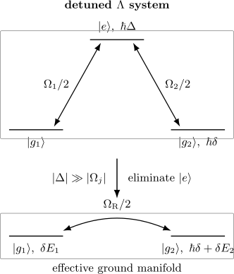
When $\lvert\Delta\rvert$ dominates the Rabi frequencies and slow ground-manifold scales, the excited amplitude is weak and fast. Eliminating $\lvert e\rangle$ leaves a Raman coupling between $\lvert g_1\rangle$ and $\lvert g_2\rangle$ together with state-dependent ac Stark shifts.

For

$$\lvert\Psi\rangle = c_1\lvert g_1\rangle + c_2\lvert g_2\rangle + c_e\lvert e\rangle,$$

the amplitude equations are

$$\begin{aligned} i\dot c_1 &= \frac{\Omega_1^*}{2}c_e, \\ i\dot c_2 &= \delta c_2 + \frac{\Omega_2^*}{2}c_e, \\ i\dot c_e &= \Delta c_e + \frac{\Omega_1c_1+\Omega_2c_2}{2}. \end{aligned}$$

If

$$\lvert\Omega_1\rvert, \lvert\Omega_2\rvert, \lvert\delta\rvert \ll \lvert\Delta\rvert,$$

the leading fast response is

$$c_e \simeq - \frac{ \Omega_1c_1+\Omega_2c_2 } {2\Delta}.$$

Substitution gives the ground-manifold Hamiltonian

$$\frac{H_{\mathrm{eff}}}{\hbar} = \begin{pmatrix} -\dfrac{\lvert\Omega_1\rvert^2}{4\Delta} & -\dfrac{\Omega_1^*\Omega_2}{4\Delta} \\ -\dfrac{\Omega_2^*\Omega_1}{4\Delta} & \delta-\dfrac{\lvert\Omega_2\rvert^2}{4\Delta} \end{pmatrix}.$$

The diagonal terms are ac Stark shifts. Defining the effective two-state coupling by an off-diagonal matrix element $\hbar\Omega_{\mathrm R}/2$ gives

$$\Omega_{\mathrm R} = - \frac{\Omega_1^*\Omega_2} {2\Delta}.$$

The effective two-photon detuning is

$$\delta_{\mathrm{eff}} = \delta - \frac{ \lvert\Omega_2\rvert^2 - \lvert\Omega_1\rvert^2 } {4\Delta}.$$

Thus the Raman resonance is shifted by the differential ac Stark shift. Dropping the diagonal terms while keeping the Raman coupling is inconsistent because both arise at the same order.

Bright and dark combinations

For $\delta=0$, define

$$\Omega = \sqrt{ \lvert\Omega_1\rvert^2 + \lvert\Omega_2\rvert^2 }.$$

The normalized combinations

$$\begin{aligned} \lvert B\rangle &= \frac{ \Omega_1^*\lvert g_1\rangle + \Omega_2^*\lvert g_2\rangle }{\Omega}, \\ \lvert D\rangle &= \frac{ \Omega_2\lvert g_1\rangle - \Omega_1\lvert g_2\rangle }{\Omega} \end{aligned}$$

are bright and dark, respectively. The excitation operator annihilates $\lvert D\rangle$, while

$$\begin{aligned} H_{\mathrm{eff}}\lvert B\rangle &= - \frac{\hbar\Omega^2}{4\Delta} \lvert B\rangle, \\ H_{\mathrm{eff}}\lvert D\rangle &= 0. \end{aligned}$$

The excited-state population obeys

$$\lvert c_e\rvert^2 \lesssim \frac{\Omega^2}{4\Delta^2}.$$

The dark state is exactly uncoupled for the ideal Hamiltonian, whereas the bright state acquires a virtual light shift. Time-dependent dark-state transport is a separate adiabatic-following problem; it should not be inferred from elimination alone.

Open-System Elimination

Suppose the fast excited sector also decays. Begin with a Lindblad equation,

$$\dot\rho = - \frac{i}{\hbar}[H,\rho] + \sum_k \mathcal D[L_k]\rho,$$

where

$$\mathcal D[L]\rho = L\rho L^\dagger - \frac12 \left\{ L^\dagger L,\rho \right\}.$$

Write

$$H = H_g+H_e+V_++V_-, \qquad V_-=V_+^\dagger,$$

where $V_+$ excites the slow sector into the fast one. If each $L_k$ returns population from the excited sector to the ground sector, define the excited-sector non-Hermitian Hamiltonian

$$H_{\mathrm{NH}} = H_e - \frac{i\hbar}{2} \sum_k L_k^\dagger L_k.$$

For weak excitation and an invertible fast response, the leading effective operators are

$$\begin{aligned} H_{\mathrm{eff}} &= H_g - \frac12 V_- \left[ H_{\mathrm{NH}}^{-1} + \left( H_{\mathrm{NH}}^{-1} \right)^\dagger \right] V_+, \\ L_{\mathrm{eff}}^{(k)} &= L_k H_{\mathrm{NH}}^{-1} V_+. \end{aligned}$$

They generate a trace-preserving effective master equation entirely in the retained sector:

$$\dot\rho_g = - \frac{i}{\hbar} [H_{\mathrm{eff}},\rho_g] + \sum_k \mathcal D \left[ L_{\mathrm{eff}}^{(k)} \right]\rho_g.$$

The sequence encoded by an effective jump is

$$g \xrightarrow{\,V_+\,} e \xrightarrow{\,H_{\mathrm{NH}}^{-1}\,} e \xrightarrow{\,L_k\,} g.$$

For one excited state with detuning $\Delta$ and total linewidth $\Gamma$,

$$H_{\mathrm{NH}} = \hbar \left( \Delta-\frac{i\Gamma}{2} \right) \lvert e\rangle\langle e\rvert.$$

A weak Rabi coupling $\Omega$ then produces an effective scattering scale

$$\Gamma_{\mathrm{sc}} \sim \frac{ \Gamma\lvert\Omega\rvert^2 } { 4\left[ \Delta^2+(\Gamma/2)^2 \right] }.$$

Replacing $\Delta$ by $\Delta-i\Gamma/2$ in a Hamiltonian but omitting the effective jumps describes only no-jump loss. It does not preserve trace and generally misses where the emitted population goes. Lindblad–GKSL Equation owns the master-equation structure, while Quantum-Jump Trajectories develops its conditional interpretation.

Relation to Neighboring Methods

Method	Eliminated object	Typical output	Main diagnostic
Projection methods	Complementary Hilbert subspace	Exact energy-dependent operator or memory kernel	Resolvent poles
Adiabatic elimination	Fast amplitude or rapidly relaxing sector	Local slow generator	Coupling and slow bandwidth over fast scale
Schrieffer–Wolff transformation	Weak off-diagonal block	Energy-independent block Hamiltonian and dressed observables	Coupling over spectral gap
Rotating-wave approximation	Rapidly oscillating Hamiltonian terms	Slowly varying rotating-frame Hamiltonian	Coupling over oscillation frequency
Born–Oppenheimer method	Fast coordinate-dependent eigenstates	Potential surfaces and derivative couplings	Nuclear rate over electronic gap

These methods can agree at leading order because they organize the same virtual excursions. They answer different questions:

• Use adiabatic elimination when equations of motion expose a fast response and a local slow generator is the desired output.
• Use projection methods when exact energy dependence, memory, resonances, or reconstruction is central.
• Use the Born–Oppenheimer method when slow quantum coordinates parametrize a fast eigenspace and potential surfaces plus derivative couplings are the natural output.
• Use Schrieffer–Wolff when unitary block diagonalization and consistently transformed observables are required.
• Use a full Lindblad reduction when the eliminated sector decays.

Quantum Optics and Quantum Information

Adiabatic elimination appears throughout controlled quantum systems:

• Raman qubits: an optically excited state mediates coherent transitions between long-lived states while remaining weakly populated.
• Dispersive cavity QED: a far-detuned atom or cavity mode mediates ac Stark shifts, state-dependent phases, and indirect interactions.
• Tunable couplers: an off-resonant auxiliary mode produces an effective qubit–qubit coupling, with residual population interpreted as leakage.
• Engineered dissipation: a rapidly decaying manifold produces effective pumping, cooling, or dephasing through $L_{\mathrm{eff}}^{(k)}$.
• Measurement models: a fast cavity field can follow a slower system observable, but measurement backaction and output noise must survive the reduction.

In each application, the same design tension appears. Increasing detuning suppresses unwanted fast-sector population and spontaneous scattering, but it also weakens the desired interaction. Stronger drives recover speed while eventually violating weak occupation. Gate and measurement proposals should therefore report both the effective rate and the leading leakage or scattering error.

Cavity QED provides the platform context. Two-State Hamiltonians owns the exact dynamics after a reliable two-state reduction has been obtained.

Practical Workflow

1. Choose a rotating frame or interaction picture in which the retained amplitudes are genuinely slow.
2. Identify slow and fast blocks, including every near-resonant state in the slow sector.
3. Write the exact fast solution or the equivalent Schur complement before approximating.
4. State the fast scale, coupling scale, retained bandwidth, ramp time, and intended evolution time.
5. Compute $H_{\mathrm{eff}}^{(0)}=A-BD^{-1}C$ and reconstruct the leading fast amplitude.
6. Include derivative corrections when phase accuracy, rapid ramps, or long evolution times demand them.
7. For decay, derive effective jumps as well as the coherent Hamiltonian.
8. Benchmark a small full model against the reduced dynamics, including leakage and phase error.

Common Mistakes

• Treating “unpopulated initially” as equivalent to “irrelevant dynamically.”
• Setting $\dot\psi_f=0$ before choosing a frame in which $\psi_f$ is actually fast.
• Keeping the induced off-diagonal coupling but dropping same-order energy shifts.
• Ignoring the initial transient after an abrupt switch-on.
• Using only $\lvert\Omega/\Delta\rvert\ll1$ while a two-photon detuning, ramp rate, or slow coupling is comparable with $\Delta$.
• Eliminating a near-resonant state instead of enlarging the retained sector.
• Applying a non-Hermitian substitution to an open system without effective jump operators.
• Assuming small instantaneous leakage guarantees small long-time phase error.
• Comparing effective Hamiltonian matrix elements from different frames or normalization conventions term by term.

Exercises

1. Derive the memory kernel

For constant $D$, solve

$$i\dot\psi_f = C\psi_s+D\psi_f$$

with initial value $\psi_f(t_0)$ and substitute the result into the slow equation.

Solution

Multiplication by $e^{iDt}$ gives

$$i\frac{d}{dt} \left( e^{iDt}\psi_f \right) = e^{iDt}C\psi_s.$$

Integrating from $t_0$ to $t$ yields

$$\begin{aligned} \psi_f(t) &= e^{-iD(t-t_0)} \psi_f(t_0) \\ &\quad -i\int_{t_0}^{t} e^{-iD(t-t')} C\psi_s(t')\,dt'. \end{aligned}$$

Therefore

$$\begin{aligned} i\dot\psi_s(t) &= A\psi_s(t) \\ &\quad+ Be^{-iD(t-t_0)} \psi_f(t_0) \\ &\quad -iB\int_{t_0}^{t} e^{-iD(t-t')} C\psi_s(t')\,dt'. \end{aligned}$$

The second line is the homogeneous transient and the integral is the exact memory kernel.

2. Compare with the exact two-state spectrum

Consider

$$H = \begin{pmatrix} 0 & g\\ g^* & \Delta \end{pmatrix}, \qquad \lvert g\rvert\ll\lvert\Delta\rvert.$$

Find the eliminated Hamiltonian, expand the exact eigenvalue connected to zero energy, and estimate the fast-state population.

Solution

Here $A=0$, $B=g$, $C=g^*$, and $D=\Delta$, so

$$H_{\mathrm{eff}}^{(0)} = - \frac{\lvert g\rvert^2}{\Delta}.$$

The exact root approaching zero as $g\to0$ is

$$E_s = \frac{ \Delta - \operatorname{sgn}(\Delta) \sqrt{\Delta^2+4\lvert g\rvert^2} }{2}.$$

Expansion gives

$$E_s = - \frac{\lvert g\rvert^2}{\Delta} + \frac{\lvert g\rvert^4}{\Delta^3} + O\left( \frac{\lvert g\rvert^6}{\Delta^5} \right).$$

From $E_sc_s=gc_f$,

$$\frac{c_f}{c_s} = \frac{E_s}{g} \simeq - \frac{g^*}{\Delta},$$

so the fast-state population is of order $\lvert g/\Delta\rvert^2$.

3. Recover the derivative normalization

Keep the first derivative term in

$$\psi_f = - \left( D-i\partial_t \right)^{-1} B^\dagger\psi_s$$

for a constant Hermitian block Hamiltonian. Show that the full norm induces $N=I_s+BD^{-2}B^\dagger$.

Solution

To leading order in the reconstructed fast amplitude,

$$\psi_f \simeq - D^{-1}B^\dagger\psi_s.$$

Hence

$$\begin{aligned} \lVert\Psi\rVert^2 &= \lVert\psi_s\rVert^2 + \lVert\psi_f\rVert^2 \\ &\simeq \langle\psi_s\rvert \left( I_s+BD^{-2}B^\dagger \right) \lvert\psi_s\rangle. \end{aligned}$$

Thus $N=I_s+BD^{-2}B^\dagger$. The normalized retained coordinate is $\chi=N^{1/2}\psi_s$, and the corresponding constant-block generator is symmetrized by $N^{-1/2}$ on both sides.

4. Identify the dark state

For the detuned Λ system with $\delta=0$, show that $\lvert D\rangle$ has no excited-state amplitude and find the bright-state light shift.

Solution

The excitation operator is

$$V_+ = \frac{\hbar}{2} \left( \Omega_1\lvert e\rangle\langle g_1\rvert + \Omega_2\lvert e\rangle\langle g_2\rvert \right).$$

Acting on

$$\lvert D\rangle = \frac{ \Omega_2\lvert g_1\rangle - \Omega_1\lvert g_2\rangle }{\Omega}$$

gives zero. The orthogonal bright state obeys

$$V_+\lvert B\rangle = \frac{\hbar\Omega}{2} \lvert e\rangle.$$

Therefore its second-order shift is

$$\Delta E_B = - \frac{ \lvert\hbar\Omega/2\rvert^2 }{\hbar\Delta} = - \frac{\hbar\Omega^2}{4\Delta},$$

while the dark state remains unshifted in the ideal model.

5. Tune the Raman resonance

Find the value of the bare two-photon detuning $\delta$ that makes the effective diagonal entries equal.

Solution

The diagonal difference is

$$\delta_{\mathrm{eff}} = \delta - \frac{ \lvert\Omega_2\rvert^2 - \lvert\Omega_1\rvert^2 } {4\Delta}.$$

Setting it to zero gives

$$\delta = \frac{ \lvert\Omega_2\rvert^2 - \lvert\Omega_1\rvert^2 } {4\Delta}.$$

The drive must compensate the differential, not the common, light shift.

6. Derive an effective scattering operator

A ground state $\lvert g\rangle$ couples to a decaying excited state $\lvert e\rangle$ with

$$\begin{aligned} V_+ &= \frac{\hbar\Omega}{2} \lvert e\rangle\langle g\rvert, \\ L &= \sqrt{\Gamma} \lvert g\rangle\langle e\rvert. \end{aligned}$$

Use $H_{\mathrm{NH}}=\hbar(\Delta-i\Gamma/2)\lvert e\rangle\langle e\rvert$ to find $L_{\mathrm{eff}}$ and its rate scale.

Solution

The inverse fast propagator is

$$H_{\mathrm{NH}}^{-1} = \frac{ \lvert e\rangle\langle e\rvert } {\hbar(\Delta-i\Gamma/2)}.$$

Therefore

$$L_{\mathrm{eff}} = \frac{ \sqrt{\Gamma}\,\Omega } {2(\Delta-i\Gamma/2)} \lvert g\rangle\langle g\rvert.$$

Its squared coefficient is

$$\Gamma_{\mathrm{sc}} = \frac{ \Gamma\lvert\Omega\rvert^2 } { 4\left[ \Delta^2+(\Gamma/2)^2 \right] }.$$

If another ground state is unaffected by the drive, this projector-valued jump dephases superpositions relative to that state even though it returns population to $\lvert g\rangle$.

Cross-Links

• Effective Hamiltonians and Scale Separation
• Projection Methods
• Schrieffer–Wolff Transformation
• Rotating-Wave Approximation
• Interaction Picture
• Small Parameters and Error Estimates
• Lindblad–GKSL Equation
• Quantum-Jump Trajectories
• Cavity QED
• Two-State Hamiltonians
• Adiabatic Theorem
• STIRAP

References

1. E. Brion, L. H. Pedersen, and K. Mølmer, “Adiabatic elimination in a lambda system,” Journal of Physics A: Mathematical and Theoretical 40, 1033–1043 (2007).
2. V. Paulisch, R. Han, H. K. Ng, and B.-G. Englert, “Beyond adiabatic elimination: A hierarchy of approximations for multi-photon processes,” European Physical Journal Plus 129, 12 (2014).
3. I. L. Egusquiza, “Beyond adiabatic elimination: Systematic expansions,” arXiv:1309.0628 (2013).
4. F. Reiter and A. S. Sørensen, “Effective operator formalism for open quantum systems,” Physical Review A 85, 032111 (2012).
5. L. Bouten and A. Silberfarb, “Adiabatic elimination in quantum stochastic models,” Communications in Mathematical Physics 283, 491–505 (2008).
6. D. F. V. James and J. Jerke, “Effective Hamiltonian theory and its applications in quantum information,” Canadian Journal of Physics 85, 625–632 (2007).
7. C. Cohen-Tannoudji, J. Dupont-Roc, and G. Grynberg, Atom–Photon Interactions: Basic Processes and Applications, Wiley (1992).
8. S. Bravyi, D. P. DiVincenzo, and D. Loss, “Schrieffer–Wolff transformation for quantum many-body systems,” Annals of Physics 326, 2793–2826 (2011).