STIRAP

Stimulated Raman adiabatic passage (STIRAP) transfers population between two quantum states by adiabatically rotating a dark superposition while keeping a lossy intermediate state ideally unoccupied. A pump field couples the initial state to the intermediate state, and a Stokes field couples the target state to the same intermediate state.

The defining feature is the counterintuitive pulse order: the Stokes field acts first, before there is population in the target state. During the pulse overlap, the instantaneous dark state changes continuously from the initial state to the target state:

$$|D(t)\rangle = \cos\theta(t)|1\rangle - \sin\theta(t)|2\rangle,$$

with

$$\tan\theta(t) = \frac{ \Omega_P(t) }{ \Omega_S(t) }.$$

If nonadiabatic coupling, two-photon detuning, decoherence, and unwanted levels are sufficiently small, an initial $|1\rangle$ follows this dark path to $-|2\rangle$.

STIRAP is robust against moderate pulse-area variation after the adiabaticity margin is large. It is not immune to relative phase noise, two-photon detuning, inadequate overlap, intermediate-state loss, lower-state dephasing, differential light shifts, or multilevel interference. “No intermediate population” is an ideal limiting statement, not a license to omit the loss model.

Canonical Scope

This page owns:

1. the time-dependent three-state Λ Hamiltonian for pump and Stokes fields;
2. instantaneous dark and bright states;
3. counterintuitive pulse ordering and endpoint mapping;
4. local and global adiabaticity criteria;
5. Gaussian-pulse examples and transfer diagnostics;
6. one- and two-photon detuning, optical phase, and decoherence;
7. the relation to far-detuned Raman transfer and adiabatic elimination;
8. multilevel, molecular, solid-state, and quantum-control applications.

Nearby canonical homes remain distinct:

• Electromagnetically Induced Transparency owns static weak-probe susceptibility, transparency bandwidth, slow light, and dark-state-polariton storage.
• Adiabatic Approximation owns the general time-dependent theorem, phase structure, and error estimates.
• Raman Spectroscopy owns Raman shifts, scattering observables, and molecular spectroscopic interpretation.
• Adiabatic Elimination owns the general projection of fast virtual states into effective Hamiltonians.
• Optimal Control owns objective-based numerical pulse design and constrained optimization.

This page derives STIRAP itself and cross-links rather than reproducing those general frameworks.

Three-State Model

State labels

Use:

• $|1\rangle$ for the initially populated terminal state;
• $|2\rangle$ for the desired terminal state;
• $|3\rangle$ for the radiative or otherwise lossy intermediate state.

The labels match the Λ convention on the EIT page: $|1\rangle$ and $|2\rangle$ are the two terminal states, while $|3\rangle$ is the shared intermediate.

The pump field couples

$$|1\rangle \longleftrightarrow |3\rangle$$

with Rabi frequency $\Omega_P(t)$. The Stokes field couples

$$|2\rangle \longleftrightarrow |3\rangle$$

with Rabi frequency $\Omega_S(t)$.

The name “Stokes” comes from the Raman frequency ordering. Its field can be present before target-state population exists; the protocol does not require ordinary stimulated emission from an already occupied $|2\rangle$.

Detunings

Let

$$\Delta_P = \omega_{31}-\omega_P, \qquad \Delta_S = \omega_{32}-\omega_S$$

be atom-minus-field detunings. Define

$$\Delta \equiv \Delta_P,$$

and the two-photon detuning

$$\delta = \Delta_P-\Delta_S.$$

Two-photon resonance means

$$\omega_P-\omega_S = \omega_{21}.$$

Frequencies, detunings, couplings, and decay rates are angular quantities unless divided by $2\pi$.

Rotating-frame Hamiltonian

Choose local state phases so the pulse envelopes are real and nonnegative. In the ordered basis

$$\left( |1\rangle, |2\rangle, |3\rangle \right),$$

the rotating-wave Hamiltonian is. Suppressing the explicit time arguments inside the matrix,

$$\frac{H(t)}{\hbar} = \begin{pmatrix} 0 & 0 & \Omega_P/2 \\ 0 & \delta & \Omega_S/2 \\ \Omega_P/2 & \Omega_S/2 & \Delta \end{pmatrix}.$$

This minimal model assumes:

1. the selected states and polarizations isolate one effective Λ system;
2. both rotating-wave approximations are controlled;
3. field envelopes vary slowly relative to the optical carriers;
4. spatial motion and ensemble inhomogeneity are either negligible or modeled separately;
5. dissipation is specified rather than inferred from a non-Hermitian Hamiltonian alone.

Instantaneous Dark State

Mixing angle

At exact two-photon resonance,

$$\delta=0,$$

define the generalized coupling

$$\Omega(t) = \sqrt{ \Omega_P^2(t) + \Omega_S^2(t) }.$$

The mixing angle is

$$\begin{aligned} \sin\theta(t) &= \frac{\Omega_P(t)}{\Omega(t)}, \\ \cos\theta(t) &= \frac{\Omega_S(t)}{\Omega(t)}. \end{aligned}$$

The dark and bright terminal-state superpositions are

$$\begin{aligned} |D(t)\rangle &= \cos\theta(t)|1\rangle - \sin\theta(t)|2\rangle, \\ |B(t)\rangle &= \sin\theta(t)|1\rangle + \cos\theta(t)|2\rangle. \end{aligned}$$

Direct multiplication gives

$$H(t)|D(t)\rangle=0.$$

The intermediate-state amplitudes cancel:

$$\frac{\hbar}{2} \left[ \Omega_P\cos\theta - \Omega_S\sin\theta \right] = 0.$$

Bright eigenvalues

In the basis

$$\left( |D\rangle, |B\rangle, |3\rangle \right),$$

the resonant two-photon Hamiltonian is

$$\frac{H}{\hbar} = \begin{pmatrix} 0 & 0 & 0 \\ 0 & 0 & \Omega/2 \\ 0 & \Omega/2 & \Delta \end{pmatrix}.$$

The bright eigenvalues are

$$\lambda_\pm = \frac{ \Delta \pm \sqrt{ \Delta^2+\Omega^2 } }{ 2 }.$$

At one-photon resonance,

$$\Delta=0,$$

they reduce to

$$\lambda_\pm = \pm\frac{\Omega}{2}.$$

One convenient eigenvector convention is

$$|\pm\rangle = \frac{ |B\rangle \pm |3\rangle }{ \sqrt2 }$$

at $\Delta=0$.

The instantaneous dark state has zero dynamical eigenvalue in this gauge. Its time dependence still produces geometric and nonadiabatic terms.

Counterintuitive Pulse Order

Endpoint mapping

For transfer from $|1\rangle$ to $|2\rangle$, require the asymptotic ratios

$$\frac{ \Omega_P }{ \Omega_S } \longrightarrow 0$$

at the beginning of the interaction, and

$$\frac{ \Omega_S }{ \Omega_P } \longrightarrow 0$$

at the end.

Then

$$|D(t_i)\rangle \simeq |1\rangle,$$

while

$$|D(t_f)\rangle \simeq -|2\rangle.$$

The Stokes pulse must therefore precede the pump pulse. During their overlap, $\theta$ rotates from $0$ to $\pi/2$.

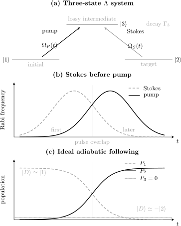
Top: the pump couples the initial state $|1\rangle$ to the lossy intermediate $|3\rangle$, while the Stokes field couples the target $|2\rangle$ to $|3\rangle$. Middle: the Stokes pulse arrives first and overlaps the later pump pulse. Bottom: adiabatic following rotates the dark state from $|1\rangle$ to $-|2\rangle$ while the ideal intermediate population remains zero.

Why the intuitive order fails

If the pump arrives first, the initial state is directly coupled to $|3\rangle$ before a dark superposition aligned with $|1\rangle$ exists. The system can undergo ordinary Rabi excitation, spontaneous loss, or detuning-sensitive Raman dynamics.

An intuitive sequence can still transfer population under specially chosen pulse areas or detunings. That transfer is not the defining dark-state adiabatic path of STIRAP.

Overlap is essential

“Stokes first” does not mean two nonoverlapping pulses. If both couplings are negligible while the mixing angle must rotate, the bright–dark gap closes and adiabatic following fails. Useful sequences have:

• a Stokes-leading entrance;
• substantial simultaneous coupling during rotation;
• a pump-dominated exit.

If the pulses overlap almost completely with a nearly constant ratio, the angle barely changes and little endpoint transfer occurs. If their separation is too large, the gap collapses between them.

Endpoint degeneracy

Both fields eventually vanish, so all bare terminal states become degenerate in the rotating interaction Hamiltonian. The elementary nondegenerate adiabatic theorem cannot be applied blindly at $t\to\pm\infty$.

The practical statement is about a finite interval: one pulse dominates while the state is aligned with a decoupled endpoint, the mixing angle rotates only while a sufficient gap exists, and the state is frozen into the target before the remaining field vanishes.

Adiabaticity

Geometric coupling

The instantaneous basis transformation contributes

$$H_{\mathrm{geom}} = - i\hbar U^\dagger\dot U.$$

At $\Delta=\delta=0$,

$$\frac{H_{\mathrm{ad}}}{\hbar} = \begin{pmatrix} 0 & -i\dot\theta/\sqrt2 & -i\dot\theta/\sqrt2 \\ i\dot\theta/\sqrt2 & \Omega/2 & 0 \\ i\dot\theta/\sqrt2 & 0 & -\Omega/2 \end{pmatrix}$$

in the basis $(|D\rangle,|+\rangle,|-\rangle)$, up to basis-phase conventions. The physically invariant magnitudes are

$$\left| \langle\pm|\dot D\rangle \right| = \frac{ |\dot\theta| }{ \sqrt2 }.$$

Nonadiabatic transfer out of the dark state is suppressed when these couplings are small relative to the bright gaps.

Mixing-angle derivative

Differentiating

$$\tan\theta = \frac{\Omega_P}{\Omega_S}$$

gives

$$\dot\theta = \frac{ \Omega_S\dot\Omega_P - \Omega_P\dot\Omega_S }{ \Omega_P^2+\Omega_S^2 }.$$

For resonant STIRAP, an exact local dimensionless ratio is

$$\epsilon_{\mathrm{ad}}(t) = \frac{ \sqrt2|\dot\theta(t)| }{ \Omega(t) }.$$

A useful requirement is

$$\max_t \epsilon_{\mathrm{ad}}(t) \ll 1.$$

The factor $\sqrt2$ depends on the chosen bright-state convention, while the scale comparison

$$|\dot\theta| \ll \Omega$$

is universal for the resonant three-state model.

Global pulse-area criterion

A common global diagnostic is

$$\mathcal S = \int \Omega(t) \,dt \gg 1.$$

Large generalized pulse area is helpful but not sufficient. A sequence can have large area and still fail because:

• the pulse ratio has the wrong endpoint order;
• the angle rotates where $\Omega$ is small;
• two-photon detuning couples dark and bright states;
• phase noise changes the dark vector;
• an unwanted level closes the relevant gap.

Local and global checks should be reported together.

Gaussian Pulse Pair

Delayed envelopes

Consider equal-peak Gaussian pulses:

$$\Omega_S(t) = \Omega_0 \exp \left[ - \frac{ \left( t+\tau/2 \right)^2 }{ 2\sigma^2 } \right],$$

and

$$\Omega_P(t) = \Omega_0 \exp \left[ - \frac{ \left( t-\tau/2 \right)^2 }{ 2\sigma^2 } \right].$$

For $\tau>0$, the Stokes pulse is centered at $-\tau/2$ and the pump at $+\tau/2$.

Their ratio is

$$\frac{\Omega_P}{\Omega_S} = \exp \left( \frac{ t\tau }{ \sigma^2 } \right).$$

Therefore

$$\theta(t) = \arctan \left[ \exp \left( \frac{ t\tau }{ \sigma^2 } \right) \right].$$

The angle derivative is

$$\dot\theta(t) = \frac{ \tau }{ 2\sigma^2 } \operatorname{sech} \left( \frac{ t\tau }{ \sigma^2 } \right).$$

Its maximum occurs at $t=0$:

$$\dot\theta_{\max} = \frac{\tau}{2\sigma^2}.$$

The generalized coupling there is

$$\Omega(0) = \sqrt2\, \Omega_0 \exp \left( - \frac{ \tau^2 }{ 8\sigma^2 } \right).$$

The center adiabatic ratio is consequently

$$\epsilon_{\mathrm{ad}}(0) = \frac{ \tau }{ 2\Omega_0\sigma^2 } \exp \left( \frac{ \tau^2 }{ 8\sigma^2 } \right).$$

This expression displays the pulse-separation tradeoff. Larger $\tau$ improves endpoint ordering but reduces overlap and the central gap.

Ideal populations

If the state follows $|D(t)\rangle$ exactly,

$$\begin{aligned} P_1(t) &= \cos^2\theta(t), \\ P_2(t) &= \sin^2\theta(t), \\ P_3(t) &= 0. \end{aligned}$$

For the Gaussian pair,

$$P_2(t) = \frac{ 1 }{ 1+ \exp \left( - \frac{ 2t\tau }{ \sigma^2 } \right) }.$$

The logistic form is the ideal adiabatic path, not a prediction that remains exact under finite detuning and decay.

Detuning Sensitivity

One-photon detuning

At $\delta=0$, the algebraic dark state remains exact for any common one-photon detuning $\Delta$. One-photon detuning is therefore less destructive than two-photon detuning in the ideal model.

It still changes the bright gaps:

$$\lambda_\pm = \frac{ \Delta \pm \sqrt{ \Delta^2+\Omega^2 } }{ 2 }.$$

For

$$|\Delta|\gg\Omega,$$

the nearest bright eigenvalue has magnitude

$$|\lambda_{\mathrm{near}}| \simeq \frac{ \Omega^2 }{ 4|\Delta| }.$$

Large one-photon detuning can therefore make adiabatic following harder by shrinking the nearest gap, even though it suppresses direct intermediate excitation in a far-detuned Raman picture.

Two-photon detuning

The term

$$\hbar\delta |2\rangle\langle2|$$

is not diagonal in the dark–bright basis. Since

$$|2\rangle = - \sin\theta|D\rangle + \cos\theta|B\rangle,$$

it contributes

$$\begin{aligned} \frac{H_\delta}{\hbar} &= \delta\sin^2\theta |D\rangle\langle D| \\ &\quad + \delta\cos^2\theta |B\rangle\langle B| \\ &\quad - \delta\sin\theta\cos\theta \left( |D\rangle\langle B| + |B\rangle\langle D| \right). \end{aligned}$$

The dark–bright coupling is largest near $\theta=\pi/4$:

$$\left| \frac{ \delta\sin2\theta }{ 2 } \right| \le \frac{|\delta|}{2}.$$

Two-photon detuning therefore directly spoils the decoupling. The allowed detuning depends on pulse duration and gap; there is no universal bandwidth independent of pulse shape.

Differential light shifts

Off-resonant couplings produce time-dependent terminal-state shifts. The effective two-photon detuning becomes

$$\delta_{\mathrm{eff}}(t) = \delta + \Delta_{\mathrm{LS},1}(t) - \Delta_{\mathrm{LS},2}(t).$$

Because the pump and Stokes intensities change differently in time, $\delta_{\mathrm{eff}}$ can sweep during the passage. Chirp compensation, polarization choice, auxiliary fields, or an expanded multilevel model may be required.

Optical Phase and Coherence

Complex couplings

Write

$$\Omega_P = |\Omega_P|e^{i\phi_P}, \qquad \Omega_S = |\Omega_S|e^{i\phi_S}.$$

With a consistent interaction-Hamiltonian convention, the dark state can be written

$$|D\rangle = \cos\theta|1\rangle - e^{i\phi} \sin\theta|2\rangle,$$

where

$$\phi = \phi_P-\phi_S.$$

Ideal complete transfer produces

$$|1\rangle \longrightarrow - e^{i\phi} |2\rangle.$$

For a pure target population this phase is global. It becomes observable when STIRAP prepares a superposition, forms one arm of an interferometer, or is embedded in a gate sequence.

Phase noise

A time-dependent relative phase contributes geometric coupling and behaves like a fluctuating two-photon detuning. The dark-state derivative contains

$$\frac{d}{dt}|D\rangle \supset - i\dot\phi\, e^{i\phi} \sin\theta |2\rangle.$$

Phase locking and optical-path stability are therefore part of the Hamiltonian control, not merely laser housekeeping.

For spatially separated beams, the relative phase also includes

$$\left( \mathbf k_P-\mathbf k_S \right) \mathbin{\cdot} \mathbf r.$$

Motion through that phase pattern creates two-photon Doppler shifts and ensemble dephasing.

Dissipation and Transfer Error

Intermediate-state decay

Let the intermediate population decay at rate $\Gamma_3$. A minimal master equation is

$$\dot\rho = - \frac{i}{\hbar} [H,\rho] + \sum_j \mathcal D[L_j]\rho,$$

with

$$\mathcal D[L]\rho = L\rho L^\dagger - \frac12 \left\{ L^\dagger L, \rho \right\}.$$

If $P_3(t)$ is small, a useful first loss estimate is

$$P_{\mathrm{surv}} \simeq \exp \left[ - \Gamma_3 \int P_3(t) \,dt \right].$$

Nonadiabatic corrections commonly give

$$P_3 = O \left[ \left( \frac{\dot\theta}{\Omega} \right)^2 \right]$$

on resonance, with pulse-shape-dependent coefficients.

Even a small peak intermediate population can cause appreciable loss if $\Gamma_3$ is large or the passage is long.

Terminal-state decoherence

The dark state is a coherence between $|1\rangle$ and $|2\rangle$. Dephasing of that coherence acts directly even when $P_3=0$. If the terminal coherence decays at rate $\gamma_{12}$, making the protocol arbitrarily slow is not beneficial.

The useful operating window is schematically

$$\frac1{\Delta_{\mathrm{gap}}} \ll T \ll \frac1{\gamma_{12}},$$

where $T$ is the passage time and $\Delta_{\mathrm{gap}}$ is the relevant minimum bright–dark gap. The first inequality is adiabatic; the second limits accumulated dephasing.

Branching and repumping

Spontaneous emission from $|3\rangle$ may return population to $|1\rangle$, to $|2\rangle$, or to states outside the modeled Λ system. A high final $|2\rangle$ population after many attempts does not prove coherent STIRAP if optical pumping can produce the same result.

Time-resolved intermediate fluorescence, reversal tests, phase-sensitive measurements, and master-equation fits help separate coherent passage from dissipative accumulation.

Far-Detuned Raman Limit

Eliminating the intermediate amplitude

For

$$|\Delta| \gg |\Omega_P|, |\Omega_S|, |\delta|,$$

the intermediate amplitude approximately follows the terminal amplitudes:

$$c_3 \simeq - \frac{ \Omega_Pc_1+\Omega_Sc_2 }{ 2\Delta }.$$

Define the pump and Stokes light-shift scales and the effective Raman coupling by

$$\begin{aligned} S_P &= \frac{\Omega_P^2}{4\Delta}, \\ S_S &= \frac{\Omega_S^2}{4\Delta}, \\ \Omega_{\mathrm{eff}} &= - \frac{\Omega_P\Omega_S}{2\Delta}. \end{aligned}$$

Substitution gives the compact effective terminal-state Hamiltonian

$$\frac{H_{\mathrm{eff}}}{\hbar} = \begin{pmatrix} - S_P & \Omega_{\mathrm{eff}}/2 \\ \Omega_{\mathrm{eff}}/2 & \delta - S_S \end{pmatrix}.$$

The same elimination generates differential AC Stark shifts. Dropping those diagonal terms while retaining the Raman coupling gives an inconsistent resonance condition.

Relation to STIRAP

Far-detuned Raman transfer and STIRAP overlap but are not synonyms.

• STIRAP emphasizes adiabatic following of a dark eigenstate and can operate near one-photon resonance.
• Adiabatic elimination emphasizes a virtual intermediate state at large detuning and produces an effective two-state model.
• A far-detuned pulse sequence can be both adiabatically eliminated and STIRAP-like if it follows the appropriate instantaneous eigenstate.
• A resonant $\pi$ pulse of the effective Raman coupling is not STIRAP merely because two fields are used.

The approximation hierarchy should be stated explicitly.

Robustness and Its Limits

What amplitude robustness means

Once

$$\epsilon_{\mathrm{ad}}\ll1,$$

moderate common rescaling of both pulse amplitudes leaves the endpoint dark state unchanged and often leaves transfer near unity. This is the familiar plateau of STIRAP efficiency versus pulse area.

The plateau has boundaries. Reducing intensity eventually violates adiabaticity; increasing it can activate off-resonant levels, ionization, AC Stark shifts, power broadening, heating, or technical nonlinearities.

Timing robustness

Transfer can tolerate a range of pulse delays when:

• Stokes still leads;
• overlap remains substantial;
• the angle rotates while the gap is large;
• endpoint ratios remain well separated.

Timing is not irrelevant. A scan over delay is one of the most useful experimental diagnostics because STIRAP should show a broad counterintuitive-order transfer region distinct from the intuitive order.

Detuning robustness

STIRAP is commonly more tolerant of one-photon detuning than two-photon detuning. The statement is qualitative. Large one-photon detuning shrinks the nearest gap, and multilevel systems can contain accidental resonances. The transfer map should be measured or simulated across both detuning axes.

Shortcuts to adiabaticity

Counterdiabatic or superadiabatic protocols add controls designed to cancel nonadiabatic transitions. In the three-state problem, the exact counterdiabatic term can require direct coupling between $|1\rangle$ and $|2\rangle$, a transition that may be forbidden or technically difficult.

Shortcuts can reduce duration, but they introduce calibration, bandwidth, phase, and model-dependence costs. They belong to the broader Optimal Control landscape rather than replacing the baseline STIRAP criteria.

Multilevel Systems

Unwanted intermediate states

Atoms and molecules rarely contain one isolated intermediate state. If several states $|3,\alpha\rangle$ participate, each has pump and Stokes couplings:

$$\Omega_{P,\alpha} \propto \langle3,\alpha| \mathbf d \mathbin{\cdot} \boldsymbol\epsilon_P |1\rangle,$$

and

$$\Omega_{S,\alpha} \propto \langle3,\alpha| \mathbf d \mathbin{\cdot} \boldsymbol\epsilon_S |2\rangle.$$

A common dark vector exists only if the coupling vectors have the required linear dependence. Additional levels can:

• create several dark states;
• remove the exact dark state;
• produce destructive transfer interference;
• shift the two-photon resonance;
• open leakage channels.

The nearest-level rule is insufficient when a farther state has a much larger transition moment.

Degenerate terminal manifolds

Zeeman, hyperfine, rotational, or vibrational degeneracy can turn one target into a manifold. Polarization and magnetic fields select which coherent superposition is transferred. Unresolved target states can make a population measurement appear efficient while reducing state fidelity.

A controlled calculation should specify:

1. quantization axis and field geometry;
2. polarization components;
3. all relevant Clebsch–Gordan or molecular line-strength factors;
4. differential shifts and decoherence;
5. preparation and detection efficiencies for each sublevel.

Continuum and lossy targets

STIRAP ideas extend to ionization, dissociation, waveguides, cavities, and continuum-assisted transfer, but a normalizable dark eigenstate and adiabatic gap may not survive unchanged. Effective non-Hermitian eigenvectors require biorthogonal analysis and a complete accounting of jump channels.

The three-state unitary formulas should be treated as a model, not a universal theorem about every delayed-pulse transfer.

Molecular Applications

Rovibrational state transfer

Molecules provide dense rovibronic structure and terminal states separated by large changes in vibrational or rotational character. STIRAP can connect an initially accessible state to a deeply bound target through an electronically excited intermediate while suppressing spontaneous emission.

The practical design problem includes:

• Franck–Condon factors for both legs;
• rotational and parity selection rules;
• intermediate-state lifetime;
• nearby rovibronic levels;
• laser phase coherence across the Raman difference;
• differential AC Stark shifts;
• spatially varying pulse ratio in a molecular sample.

Large one-leg transition strength is not enough. Both pump and Stokes matrix elements must support an adequate gap during overlap.

Ultracold molecule preparation

STIRAP is widely used to convert weakly bound atom-pair molecules into a selected rovibrational ground state. High transfer efficiency is crucial because spontaneous scattering heats or removes particles, while imperfect state purity complicates dipolar-collision and many-body experiments.

A round-trip transfer measurement can reduce some number-calibration uncertainties, but it yields the product of forward and reverse efficiencies only under a validated symmetric model.

Coherent reaction control

More elaborate adiabatic-passage networks can steer population among vibrational states or reaction channels. Claims of chemical selectivity must distinguish coherent pathway control from ordinary spectral selection, heating, and state-dependent detection.

Quantum Platforms and Applications

Atomic state preparation

STIRAP can transfer population among hyperfine, Zeeman, metastable, and Rydberg states. Uses include preparation, shelving, readout, coherent beam splitters, and loading of states with weak direct transitions.

Cavity and photon interfaces

In cavity-assisted variants, one leg can be a quantized cavity coupling. Adiabatic following can map an atomic excitation to a cavity photon or vice versa while suppressing occupation of a lossy excited atomic state. Cavity leakage, cooperativity, wave-packet shaping, and input–output boundary conditions then enter.

Cavity QED owns the open cavity framework.

Solid-state and circuit systems

Quantum dots, defect centers, superconducting circuits, and mechanical or photonic mode networks can implement STIRAP-like Hamiltonians. Their selection rules, anharmonicity, drive cross-coupling, and decoherence differ from atomic Λ systems.

In a ladder circuit, the “intermediate” may not be the most lossy state, and strong microwave drives can address unintended transitions. State tomography and full multilevel simulations are therefore especially useful.

Superposition preparation

If the pulse ratio approaches a finite value instead of infinity at the end, fractional STIRAP can prepare

$$|\psi_f\rangle = \cos\theta_f|1\rangle - e^{i\phi_f} \sin\theta_f|2\rangle.$$

This turns pulse-ratio and optical-phase control into amplitude and phase control. Unlike complete transfer, the relative phase is directly observable.

A Reliable Analysis Workflow

1. Draw the real coupling graph. Include all levels within relevant detunings and strong-coupling scales.
2. State the local labels and conventions. Identify initial, target, intermediate, pump, Stokes, $\Omega/2$, and detuning signs.
3. Verify the instantaneous dark vector. Check cancellation using complex matrix elements, not only scalar pulse envelopes.
4. Plot pulse ratio and generalized gap. Pulse intensity plots alone do not show where the angle rotates.
5. Evaluate local adiabaticity. Compute $|\dot\theta|$ and the actual nearest complex gap.
6. Scan both pulse orders. A counterintuitive-order plateau is a key diagnostic.
7. Map one- and two-photon detuning. Include time-dependent light shifts and Doppler terms.
8. Model dissipation with a master equation. Include branching, dephasing, and leakage.
9. Calibrate preparation and detection. Separate transfer fidelity from state-dependent counting efficiency.
10. Test round trips and phases when possible. Population alone may not establish coherent transfer.
11. Report uncertainty and model discrepancy. Include pulse shape, timing, local field, polarization, and multilevel sensitivity.

Common Mistakes

Calling any delayed Raman pair STIRAP

STIRAP requires dark-state adiabatic following with the counterintuitive ratio change. Two delayed fields can instead drive ordinary Raman Rabi oscillations, chirped passage, or incoherent pumping.

Thinking Stokes first means no pulse overlap

The angle must rotate while a bright–dark gap is open. Substantial overlap is essential.

Using only a pulse-area criterion

A large $\int\Omega\,dt$ does not guarantee correct endpoint ratios, local adiabaticity, or two-photon resonance.

Claiming exactly zero intermediate population

Finite-speed, detuned, decohering, and multilevel protocols have nonzero intermediate admixture. Its time integral, not only its peak, controls spontaneous loss.

Assuming one-photon detuning is harmless

It preserves the ideal dark vector at $\delta=0$ but can shrink the nearest gap and activate spectator states.

Ignoring differential AC Stark shifts

The same strong pulses that create the gap can move the two-photon resonance during the passage.

Treating terminal-state phase as irrelevant

It is global only for complete transfer into one isolated target. It matters for superpositions, interference, gates, and reverse passage.

Confusing robust with insensitive

STIRAP has parameter plateaus, not universal immunity. Phase noise, two-photon detuning, decoherence, and level crowding remain limiting.

Inferring coherent efficiency from final population alone

Optical pumping and branching can populate the target. Pulse-order scans, reversal, phase tests, and time-resolved loss constrain alternatives.

Applying a three-state model to a dense molecule without audit

Several intermediate levels can interfere, shift, or eliminate the desired dark path. Molecular line strengths and parity must be included.

Key Results

For

$$\frac{H(t)}{\hbar} = \begin{pmatrix} 0 & 0 & \Omega_P/2 \\ 0 & \delta & \Omega_S/2 \\ \Omega_P/2 & \Omega_S/2 & \Delta \end{pmatrix},$$

the exact dark state at $\delta=0$ is

$$|D(t)\rangle = \frac{ \Omega_S(t)|1\rangle - \Omega_P(t)|2\rangle }{ \sqrt{ \Omega_P^2(t)+\Omega_S^2(t) } }.$$

Counterintuitive endpoint ordering gives

$$|D(t_i)\rangle \simeq |1\rangle, \qquad |D(t_f)\rangle \simeq -|2\rangle.$$

The mixing-angle derivative is

$$\dot\theta = \frac{ \Omega_S\dot\Omega_P - \Omega_P\dot\Omega_S }{ \Omega_P^2+\Omega_S^2 }.$$

At one-photon resonance, a useful local criterion is

$$\epsilon_{\mathrm{ad}} = \frac{ \sqrt2|\dot\theta| }{ \sqrt{ \Omega_P^2+\Omega_S^2 } } \ll 1.$$

For common one-photon detuning, the bright eigenvalues are

$$\lambda_\pm = \frac{ \Delta \pm \sqrt{ \Delta^2+\Omega_P^2+\Omega_S^2 } }{ 2 }.$$

Further Connections

• Dressed States supplies the instantaneous eigenbasis and avoided-crossing language.
• Rabi Oscillations gives the pulse-area-sensitive coherent transfer that STIRAP is often compared against.
• Quantum Control in AMO places dark-state passage in a method-selection map with resonant, composite, optimal, and feedback control.
• Landau–Zener Transition develops nonadiabatic transitions near an avoided crossing.
• Adiabatic Theorem records the general spectral-gap and matrix-element statement.
• Nonadiabatic Coupling develops molecular derivative couplings and breakdown of adiabatic separation.
• Cold Molecules places STIRAP inside the atom-pair association, trapping, survival, and reverse-transfer readout pipeline.
• Precision Spectroscopy supplies detuning calibration, systematic-shift, and uncertainty methods.

References

1. U. Gaubatz, P. Rudecki, S. Schiemann, and K. Bergmann, “Population transfer between molecular vibrational levels by stimulated Raman scattering with partially overlapping laser fields,” Journal of Chemical Physics 92, 5363–5376 (1990).
2. K. Bergmann, H. Theuer, and B. W. Shore, “Coherent population transfer among quantum states of atoms and molecules,” Reviews of Modern Physics 70, 1003–1025 (1998).
3. N. V. Vitanov, A. A. Rangelov, B. W. Shore, and K. Bergmann, “Stimulated Raman adiabatic passage in physics, chemistry, and beyond,” Reviews of Modern Physics 89, 015006 (2017).
4. D. Grischkowsky and M. M. T. Loy, “Adiabatic following model for two-photon transitions: Nonlinear mixing and pulse propagation,” Physical Review A 12, 1117–1131 (1975).
5. J. Martin, B. W. Shore, and K. Bergmann, “Coherent population transfer in multilevel systems with magnetic sublevels. III. Experimental results,” Physical Review A 54, 1556–1569 (1996).
6. T. A. Laine and S. Stenholm, “Adiabatic processes in three-level systems,” Physical Review A 53, 2501–2512 (1996).
7. K. S. Kumar, A. Vepsäläinen, S. Danilin, and G. S. Paraoanu, “Stimulated Raman adiabatic passage in a three-level superconducting circuit,” Nature Communications 7, 10628 (2016).
8. K.-K. Ni et al., “A high phase-space-density gas of polar molecules,” Science 322, 231–235 (2008).
9. X. Chen and J. G. Muga, “Engineering of fast population transfer in three-level systems,” Physical Review A 86, 033405 (2012).

Exercises

1. Verify the instantaneous eigenstates

At $\delta=0$, use

$$\frac{H}{\hbar} = \begin{pmatrix} 0 & 0 & \Omega_P/2 \\ 0 & 0 & \Omega_S/2 \\ \Omega_P/2 & \Omega_S/2 & \Delta \end{pmatrix}.$$

1. Verify that $H|D\rangle=0$.
2. Transform the remaining block to the $|B\rangle,|3\rangle$ basis.
3. Find $\lambda_\pm$.

Solution

The dark vector is

$$|D\rangle = \frac1{\Omega} \begin{pmatrix} \Omega_S \\ -\Omega_P \\ 0 \end{pmatrix},$$

where

$$\Omega = \sqrt{ \Omega_P^2+\Omega_S^2 }.$$

The only nontrivial component in the multiplication is

$$\left( \frac{H}{\hbar}|D\rangle \right)_3 = \frac{ \Omega_P\Omega_S - \Omega_S\Omega_P }{ 2\Omega } = 0.$$

The first two components vanish directly, so $H|D\rangle=0$.

The bright vector is

$$|B\rangle = \frac1{\Omega} \begin{pmatrix} \Omega_P \\ \Omega_S \\ 0 \end{pmatrix}.$$

It obeys

$$\frac{H}{\hbar}|B\rangle = \frac{\Omega}{2}|3\rangle.$$

Thus

$$\frac{H_{B3}}{\hbar} = \begin{pmatrix} 0 & \Omega/2 \\ \Omega/2 & \Delta \end{pmatrix}.$$

The characteristic equation is

$$\lambda^2 - \Delta\lambda - \frac{\Omega^2}{4} = 0,$$

so

$$\lambda_\pm = \frac{ \Delta \pm \sqrt{ \Delta^2+\Omega^2 } }{ 2 }.$$

2. Analyze delayed Gaussian pulses

For

$$\Omega_S(t) = \Omega_0 \exp \left[ - \frac{ (t+\tau/2)^2 }{ 2\sigma^2 } \right],$$

and

$$\Omega_P(t) = \Omega_0 \exp \left[ - \frac{ (t-\tau/2)^2 }{ 2\sigma^2 } \right],$$

derive:

1. $\Omega_P/\Omega_S$;
2. $\theta(t)$;
3. $\dot\theta(t)$;
4. the ideal target population $P_2(t)$.

Solution

The logarithm of the pulse ratio is

$$\begin{aligned} \ln \frac{\Omega_P}{\Omega_S} &= - \frac{ (t-\tau/2)^2 - (t+\tau/2)^2 }{ 2\sigma^2 } \\ &= \frac{t\tau}{\sigma^2}. \end{aligned}$$

Therefore

$$\frac{\Omega_P}{\Omega_S} = \exp \left( \frac{t\tau}{\sigma^2} \right),$$

and

$$\theta(t) = \arctan \left[ \exp \left( \frac{t\tau}{\sigma^2} \right) \right].$$

Using

$$\frac{d}{dx}\arctan(e^x) = \frac1{2\cosh x},$$

gives

$$\dot\theta(t) = \frac{\tau}{2\sigma^2} \operatorname{sech} \left( \frac{t\tau}{\sigma^2} \right).$$

Finally,

$$\begin{aligned} P_2(t) &= \sin^2\theta(t) \\ &= \frac{ \tan^2\theta }{ 1+\tan^2\theta } \\ &= \frac{ 1 }{ 1+ \exp \left( - \frac{2t\tau}{\sigma^2} \right) }. \end{aligned}$$

For $\tau>0$, this rises from zero to one.

3. Estimate local adiabaticity

Take

$$\sigma = 1.0\ \mathrm{\mu s}, \qquad \tau = 1.2\ \mathrm{\mu s},$$

and

$$\frac{\Omega_0}{2\pi} = 10.0\ \mathrm{MHz}.$$

At the pulse midpoint:

1. calculate $\dot\theta_{\max}$;

2. calculate $\Omega(0)$;

3. calculate the local adiabaticity ratio

   $$\epsilon_{\mathrm{ad}}(0) = \frac{ \sqrt2\dot\theta_{\max} }{ \Omega(0) }.$$

Solution

The maximum angle speed is

$$\begin{aligned} \dot\theta_{\max} &= \frac{\tau}{2\sigma^2} \\ &= \frac{ 1.2\times10^{-6} }{ 2(1.0\times10^{-6})^2 } \\ &= 6.0\times10^5\ \mathrm{s^{-1}}. \end{aligned}$$

The midpoint coupling is

$$\Omega(0) = \sqrt2\, \Omega_0 \exp \left( - \frac{\tau^2}{8\sigma^2} \right).$$

Since $\tau^2/(8\sigma^2)=0.18$,

$$\begin{aligned} \Omega(0) &= \sqrt2 \left[ 2\pi(10.0\times10^6) \right] e^{-0.18} \\ &\simeq 7.42\times10^7\ \mathrm{s^{-1}}. \end{aligned}$$

Hence

$$\begin{aligned} \epsilon_{\mathrm{ad}}(0) &= \frac{ \sqrt2(6.0\times10^5) }{ 7.42\times10^7 } \\ &\simeq 0.0114. \end{aligned}$$

The midpoint is strongly adiabatic by this local criterion. A complete assessment still checks the pulse wings, detuning, and decoherence.

4. See how one-photon detuning shrinks the gap

At one instant, suppose

$$\frac{\Omega}{2\pi} = 10\ \mathrm{MHz}.$$

Compare the nearest bright–dark gap for:

1. $\Delta=0$;
2. $\Delta/(2\pi)=100\ \mathrm{MHz}$.

Use the large-detuning approximation for the second case.

Solution

At resonance,

$$\lambda_\pm = \pm\frac{\Omega}{2},$$

so the nearest gap is

$$\frac{ \Delta_{\mathrm{gap,res}} }{ 2\pi } = 5.0\ \mathrm{MHz}.$$

For large positive detuning,

$$|\lambda_{\mathrm{near}}| \simeq \frac{\Omega^2}{4|\Delta|}.$$

In frequency units,

$$\begin{aligned} \frac{ \Delta_{\mathrm{gap,far}} }{ 2\pi } &\simeq \frac{ (10\ \mathrm{MHz})^2 }{ 4(100\ \mathrm{MHz}) } \\ &= 0.250\ \mathrm{MHz}. \end{aligned}$$

The nearest gap is smaller by a factor of $20$. The ideal dark vector still exists at two-photon resonance, but the same pulse envelopes are much less adiabatic relative to this gap.

5. Track the transferred optical phase

Let

$$\phi = \phi_P-\phi_S = \frac{\pi}{3}$$

be constant during a complete STIRAP sequence.

1. What target state follows from an initial $|1\rangle$?
2. Is this phase observable in a final population measurement?
3. When would it become observable?

Solution

The complex dark state is

$$|D\rangle = \cos\theta|1\rangle - e^{i\phi} \sin\theta|2\rangle.$$

At the end of complete transfer,

$$|\psi_f\rangle = - e^{i\pi/3}|2\rangle = e^{i4\pi/3}|2\rangle.$$

For a state occupying only $|2\rangle$, this overall phase does not change the population. It becomes observable if the target interferes with a reference amplitude, if fractional STIRAP prepares a superposition, if the passage is reversed in a phase-sensitive sequence, or if STIRAP is part of a quantum gate.

Fluctuation of $\phi$ during the sequence is more serious than a fixed phase: it changes the instantaneous dark vector and can cause transfer error.

6. Estimate spontaneous loss from residual occupation

Suppose the intermediate population averages

$$\overline{P_3} = 1.0\times10^{-3}$$

during a $2.0\ \mathrm{\mu s}$ overlap. Let

$$\frac{\Gamma_3}{2\pi} = 6.0\ \mathrm{MHz}.$$

Estimate the no-jump survival and loss probabilities.

Solution

Approximate

$$\int P_3(t)\,dt \simeq \overline{P_3}T.$$

The integrated decay hazard is

$$\begin{aligned} \Lambda &= \Gamma_3\overline{P_3}T \\ &= \left[ 2\pi(6.0\times10^6) \right] \left( 1.0\times10^{-3} \right) \\ &\quad\times \left( 2.0\times10^{-6} \right) \\ &\simeq 0.0754. \end{aligned}$$

Therefore

$$P_{\mathrm{surv}} \simeq e^{-\Lambda} \simeq 0.927,$$

and

$$P_{\mathrm{loss}} \simeq 1-P_{\mathrm{surv}} \simeq 0.073.$$

An average intermediate population of only $10^{-3}$ still produces about $7\%$ loss because the radiative rate is fast on the pulse timescale.

7. Derive the far-detuned Raman Hamiltonian

For

$$|\Delta| \gg |\Omega_P|, |\Omega_S|, |\delta|,$$

start from the amplitude equations generated by the three-state Hamiltonian.

1. Set $\dot c_3\simeq0$ and solve for $c_3$.
2. Derive the effective $2\times2$ Hamiltonian.
3. Identify the effective Raman Rabi frequency and differential light shift.

Solution

The intermediate amplitude equation is

$$i\dot c_3 = \Delta c_3 + \frac{\Omega_P}{2}c_1 + \frac{\Omega_S}{2}c_2.$$

Adiabatic elimination gives

$$c_3 \simeq - \frac{ \Omega_Pc_1+\Omega_Sc_2 }{ 2\Delta }.$$

The terminal equations are

$$i\dot c_1 = \frac{\Omega_P}{2}c_3,$$

and

$$i\dot c_2 = \delta c_2 + \frac{\Omega_S}{2}c_3.$$

Introduce

$$\begin{aligned} S_P &= \frac{\Omega_P^2}{4\Delta}, \\ S_S &= \frac{\Omega_S^2}{4\Delta}, \\ \Omega_{\mathrm{eff}} &= - \frac{\Omega_P\Omega_S}{2\Delta}. \end{aligned}$$

Substitution then yields

$$\frac{H_{\mathrm{eff}}}{\hbar} = \begin{pmatrix} - S_P & \Omega_{\mathrm{eff}}/2 \\ \Omega_{\mathrm{eff}}/2 & \delta-S_S \end{pmatrix}.$$

The differential shift of the two terminal diagonal energies is

$$\Delta_{\mathrm{diff}} = \frac{ \Omega_P^2-\Omega_S^2 }{ 4\Delta }$$

up to the chosen sign for the effective two-photon detuning. It must be included when setting Raman resonance.

8. Audit a claimed STIRAP transfer

An experiment reports $92\%$ target population after two delayed pulses. The target population is also $35\%$ for the intuitive pulse order. No intermediate fluorescence, two-photon detuning map, phase-coherence measurement, or preparation/detection correction is reported.

1. Does the final population alone establish STIRAP?
2. What alternative mechanisms remain?
3. Propose a compact validation program.

Solution

The final population alone does not establish dark-state adiabatic passage. The substantial intuitive-order signal already shows that ordinary Raman Rabi transfer, direct excitation, optical pumping, or pulse-area effects may contribute.

Remaining alternatives include:

• dissipative pumping through $|3\rangle$;
• a far-detuned Raman pulse-area process;
• unresolved extra intermediate states;
• target-selective detection bias;
• spontaneous branching into the target;
• incoherent accumulation over repeated trials.

A compact validation program should:

1. scan pulse delay through counterintuitive and intuitive orders;
2. map transfer over one- and two-photon detuning;
3. vary common pulse amplitude and test for an adiabatic plateau;
4. measure or bound time-integrated intermediate fluorescence;
5. repeat at several pulse durations to test local adiabatic scaling;
6. perform reverse STIRAP and a round-trip coherence test;
7. calibrate initial preparation and state-dependent detection;
8. fit a multilevel master equation including branching and phase noise.

Evidence for STIRAP is strongest when the counterintuitive plateau, two-photon sensitivity, low intermediate loss, and coherent reversibility are all reproduced by one constrained model.

Frontier Context

Molecular Control Frontiers tracks current molecular transfer efficiencies, phase-noise limits, multilevel leakage, repeated-cycle performance, and unresolved scaling questions. The dark-state derivation, counterintuitive pulse sequence, adiabaticity criteria, detuning structure, and standard failure modes developed here remain canonical.