Electromagnetically Induced Transparency

Electromagnetically induced transparency (EIT) is the suppression of probe absorption by a coherent control field that creates destructive interference among excitation pathways. In its canonical Λ configuration, two long-lived states couple to one radiative state. At exact two-photon resonance, the interaction Hamiltonian has a superposition with no excited state component:

$$|D\rangle = \frac{ \Omega_c|1\rangle - \Omega_p|2\rangle }{ \sqrt{ \Omega_p^2+\Omega_c^2 } }.$$

This dark state cannot absorb through the modeled optical transition. The same coherence that opens a narrow transparency window also produces a steep dispersive response. A probe pulse can therefore acquire a large group delay, and an adiabatically varied control can map its envelope into a collective ground-state coherence.

These statements have conditions. Finite ground-state decoherence prevents perfect transparency. A narrow dip need not contain two split response poles. A delayed pulse is not automatically stored, and storage of a classical pulse does not by itself demonstrate a quantum memory. EIT is a coherent open-system and propagation effect, not merely a three-level eigenvector.

Canonical Scope

This page owns:

1. the Λ-system rotating-frame Hamiltonian and detuning conventions;
2. dark and bright superpositions at two-photon resonance;
3. the weak-probe optical coherence and homogeneous EIT line shape;
4. transparency depth, intrinsic width, pole splitting, and propagation bandwidth;
5. the connection between dispersion, pulse delay, and spatial compression;
6. the dark-state-polariton map underlying EIT storage;
7. Doppler, spin-wave, multilevel, optical-depth, and detector effects;
8. criteria for distinguishing EIT, coherent population trapping, and Autler–Townes splitting.

Nearby pages retain distinct responsibilities:

• Optical Bloch Equations owns the driven two-state master equation, saturation, and ordinary power broadening.
• Dressed States owns the general eigenstate, Floquet, and atom–field dressing language.
• Autler–Townes Splitting owns resolved weak-probe doublets and the split-pole criterion.
• Line Shapes and Broadening owns homogeneous, Doppler, collisional, transit, and instrumental width conventions.

STIRAP owns counterintuitive pulse ordering, time-dependent dark-state rotation, adiabatic population transfer, and its molecular-control applications. The present page discusses that connection without duplicating the transfer protocol.

Three-Level Configurations

Λ system

The canonical Λ system contains two lower states, $|1\rangle$ and $|2\rangle$, coupled to one excited state $|3\rangle$:

$$|1\rangle \longleftrightarrow |3\rangle \longleftrightarrow |2\rangle.$$

A weak probe drives $|1\rangle\leftrightarrow|3\rangle$, and a stronger control drives $|2\rangle\leftrightarrow|3\rangle$. The long lifetime of the $|1\rangle$–$|2\rangle$ coherence is the central advantage. Hyperfine, Zeeman, vibrational, spin, and solid-state sublevels can provide the two lower states.

Ladder system

A ladder or cascade has ordered energies

$$E_1<E_2<E_3,$$

with the probe on $|1\rangle\leftrightarrow|2\rangle$ and the control on $|2\rangle\leftrightarrow|3\rangle$. It can possess a coherent superposition that avoids the intermediate state, but its two-photon coherence includes the upper state and often decays faster than a Λ ground-state coherence.

The same algebra can therefore yield a transparency dip, but the linewidth, population dynamics, Doppler sign, and crossover to Autler–Townes splitting are configuration dependent. The ladder response used in Rydberg EIT belongs to the same family, not to an interchangeable relabeling of every Λ formula.

V system

A V system couples one lower state to two excited states. A superposition of excited states can be orthogonal to the optical coupling, but it is usually less protected because radiative decay acts directly on that coherence. A strong control also changes the population of the shared lower state. Spontaneously generated coherence can matter when dipoles and decay channels are not independent.

Claims about EIT in a V system therefore require its actual master equation. The canonical derivation below uses a Λ system and does not export its ground-coherence lifetime or threshold formulas unchanged.

Λ-System Hamiltonian

Frequencies and detunings

Let

$$\omega_{31} = \frac{E_3-E_1}{\hbar}, \qquad \omega_{32} = \frac{E_3-E_2}{\hbar}.$$

The probe and control angular frequencies are $\omega_p$ and $\omega_c$. Use the atom-minus-field detunings

$$\Delta_p = \omega_{31}-\omega_p, \qquad \Delta_c = \omega_{32}-\omega_c.$$

The Λ two-photon detuning is

$$\delta = \Delta_p-\Delta_c.$$

Thus

$$\delta = \omega_{21} - \left( \omega_p-\omega_c \right),$$

where $\omega_{21}=(E_2-E_1)/\hbar$. Two-photon resonance means $\omega_p-\omega_c=\omega_{21}$.

This sign differs from a ladder, where the two absorbed field frequencies add and the corresponding atom-minus-field detunings add. Frequencies, detunings, Rabi frequencies, and decay rates are angular quantities unless a factor of $2\pi$ is shown.

Rotating-frame matrix

For an open three-state chain, state phases can make the local Rabi coefficients $\Omega_p$ and $\Omega_c$ real and nonnegative. In the ordered basis

$$\left( |1\rangle, |2\rangle, |3\rangle \right),$$

the rotating-wave Hamiltonian is

$$\frac{H}{\hbar} = \begin{pmatrix} 0 & 0 & \Omega_p/2 \\ 0 & \delta & \Omega_c/2 \\ \Omega_p/2 & \Omega_c/2 & \Delta_p \end{pmatrix}.$$

The model assumes that:

1. the selected fields and states form an adequate closed coupling graph;
2. both rotating-wave approximations are controlled;
3. the probe is weak when the linear susceptibility is used;
4. dissipation can be represented by specified coherence and population rates;
5. velocity, position, polarization, and field amplitude are resolved before ensemble averaging.

A spatially varying relative optical phase cannot be discarded globally. It becomes the phase and wave vector of the stored ground-state coherence.

Dark and Bright States

Exact dark vector

At two-photon resonance,

$$\delta=0,$$

define

$$\Omega = \sqrt{ \Omega_p^2+\Omega_c^2 }.$$

The normalized dark and bright lower-state combinations are

$$\begin{aligned} |D\rangle &= \frac{ \Omega_c|1\rangle - \Omega_p|2\rangle }{ \Omega }, \\ |B\rangle &= \frac{ \Omega_p|1\rangle + \Omega_c|2\rangle }{ \Omega }. \end{aligned}$$

Direct multiplication gives

$$H|D\rangle=0.$$

The cancellation occurs in the excited-state amplitude:

$$\frac{\hbar}{2} \left( \Omega_p\Omega_c - \Omega_c\Omega_p \right) = 0.$$

By contrast,

$$H|B\rangle = \frac{\hbar\Omega}{2} |3\rangle.$$

In the basis $(|D\rangle,|B\rangle,|3\rangle)$, the resonant lower-state block separates:

$$\frac{H}{\hbar} = \begin{pmatrix} 0 & 0 & 0 \\ 0 & 0 & \Omega/2 \\ 0 & \Omega/2 & \Delta_p \end{pmatrix}.$$

The dark state is exact for any common one-photon detuning $\Delta_p$ when $\delta=0$ in this ideal Hamiltonian. Loss, differential shifts, phase noise, and additional levels spoil that statement to varying degrees.

Weak-probe limit

When

$$\Omega_p\ll\Omega_c,$$

the dark state is

$$|D\rangle \simeq |1\rangle - \frac{\Omega_p}{\Omega_c} |2\rangle.$$

Most population remains in $|1\rangle$, but the control converts a small probe-induced amplitude into a phase-coherent lower-state superposition. The vanishing excited amplitude suppresses spontaneous scattering.

This eigenvector is the closed-system core of EIT. Observable transparency, however, requires an open-system steady response and a propagation model.

What breaks darkness

The ideal cancellation is degraded by:

• nonzero two-photon detuning;
• decay or dephasing of $\rho_{12}$;
• fluctuating relative laser phase;
• differential Zeeman, Stark, or collisional shifts;
• unequal Doppler shifts;
• polarization impurities and unresolved sublevels;
• probe saturation and control-induced optical pumping;
• nonadiabatic control changes.

The relevant question is not whether an algebraic dark vector exists, but whether the prepared ensemble follows it coherently for the duration and bandwidth of the experiment.

Weak-Probe Response

Coherence rates

Let:

• $\gamma_{13}$ be the homogeneous decay rate of the optical coherence $\rho_{13}$;
• $\gamma_{12}$ be the homogeneous decay rate of the lower-state coherence $\rho_{12}$.

Both are angular-frequency HWHM parameters in the coherence equations. A simple Markovian model gives

$$\gamma_{13} = \frac{\Gamma_1+\Gamma_3}{2} + \gamma_{13}^*,$$

and

$$\gamma_{12} = \frac{\Gamma_1+\Gamma_2}{2} + \gamma_{12}^*.$$

For two stable lower states, $\Gamma_1$ and $\Gamma_2$ can be negligible, leaving laser phase noise, collisions, magnetic gradients, motion, and other pure-dephasing mechanisms. The useful hierarchy is often

$$\gamma_{12}\ll\gamma_{13}.$$

Linearized Bloch equations

Assume

$$\rho_{11}\simeq1, \qquad \rho_{22}, \rho_{33} = O(\Omega_p^2).$$

To first order in $\Omega_p$, the slowly varying coherences obey

$$\begin{aligned} \dot\rho_{13} &= - \left( \gamma_{13}-i\Delta_p \right) \rho_{13} \\ &\quad + i\frac{\Omega_p}{2} + i\frac{\Omega_c}{2}\rho_{12}, \\ \dot\rho_{12} &= - \left( \gamma_{12}-i\delta \right) \rho_{12} \\ &\quad + i\frac{\Omega_c}{2}\rho_{13}. \end{aligned}$$

In steady state,

$$\rho_{12} = \frac{ i\Omega_c\rho_{13}/2 }{ \gamma_{12}-i\delta }.$$

Substitution gives the canonical linear response:

$$\frac{\rho_{13}}{\Omega_p} = \frac{i}{2} \frac{ \gamma_{12}-i\delta }{ \left( \gamma_{13}-i\Delta_p \right) \left( \gamma_{12}-i\delta \right) + \Omega_c^2/4 }.$$

Define the positive normalized absorption proxy for this phase convention:

$$\mathcal A \left( \Delta_p,\delta \right) \equiv \operatorname{Im} \left( \frac{\rho_{13}}{\Omega_p} \right).$$

The actual susceptibility includes number density, the probe dipole matrix element, field normalization, and a sign fixed by the positive-frequency convention. Absorption and phase must be propagated from one consistent choice; changing a state phase changes intermediate coherence signs but not transmission or delay.

When $\Omega_c=0$,

$$\frac{\rho_{13}}{\Omega_p} = \frac{i}{ 2 \left( \gamma_{13}-i\Delta_p \right) },$$

and

$$\mathcal A_0(\Delta_p) = \frac{ \gamma_{13} }{ 2 \left( \Delta_p^2+\gamma_{13}^2 \right) }.$$

The control therefore modifies a line that would otherwise be one Lorentzian.

Transparency Depth and Width

Resonant control

Set

$$\Delta_c=0,$$

so that $\delta=\Delta_p$. Define

$$a = \gamma_{13}\gamma_{12} + \frac{\Omega_c^2}{4},$$

and

$$b = \gamma_{13}+\gamma_{12}.$$

The absorption proxy becomes

$$\mathcal A(\Delta_p) = \frac{ \gamma_{13}\Delta_p^2 + \gamma_{12}a }{ 2 \left[ \left( a-\Delta_p^2 \right)^2 + b^2\Delta_p^2 \right] }.$$

At line center,

$$\mathcal A(0) = \frac{ \gamma_{12} }{ 2 \left( \gamma_{13}\gamma_{12} + \Omega_c^2/4 \right) }.$$

Relative to the no-control peak,

$$\frac{ \mathcal A(0) }{ \mathcal A_0(0) } = \frac{ \gamma_{13}\gamma_{12} }{ \gamma_{13}\gamma_{12} + \Omega_c^2/4 }.$$

Perfect transparency requires $\gamma_{12}=0$ in this ideal model. Deep but imperfect transparency requires

$$\Omega_c^2 \gg 4\gamma_{13}\gamma_{12}.$$

This scale can be much smaller than the control strength required to split the response poles.

Intrinsic homogeneous window

In the narrow-window regime,

$$|\delta|, \gamma_{12}, \frac{\Omega_c^2}{4\gamma_{13}} \ll \gamma_{13},$$

the control creates an approximate transparency HWHM

$$\gamma_{\mathrm{EIT}} \simeq \gamma_{12} + \frac{\Omega_c^2}{4\gamma_{13}}.$$

The corresponding homogeneous FWHM is approximately

$$w_{\mathrm{EIT}} \simeq 2\gamma_{\mathrm{EIT}}.$$

This is a local susceptibility width, not a universal measured linewidth. Optical depth, Doppler averaging, control inhomogeneity, scan noise, and the chosen width estimator can change the observed window.

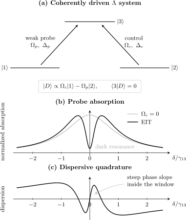
Top: a weak probe and coherent control couple two lower states to one radiative state; their dark superposition has no $|3\rangle$ component. Bottom: a representative homogeneous weak-probe response with $\gamma_{12}=0.02\gamma_{13}$ and $\Omega_c=0.8\gamma_{13}$. The absorption dip occurs even though the response poles are not split; the odd dispersive quadrature is steep inside the same narrow interval.

Optical-depth-limited bandwidth

Let $d$ be the resonant intensity optical depth without the control. A small residual absorption that looks negligible in a single-atom response can be important after propagation:

$$T(\omega_p) = \exp \left[ - d \frac{ \mathcal A(\omega_p) }{ \mathcal A_0(0) } \right]$$

for a uniform weakly dispersive sample in the simplest Beer–Lambert model.

For $\gamma_{12}=0$ and a resonant control, expansion near line center gives the propagation scale

$$\Delta\omega_{\mathrm{prop}} \sim \frac{ \Omega_c^2 }{ 4\gamma_{13}\sqrt d }.$$

The numerical factor depends on whether one uses RMS width, HWHM, $1/e$ transmission, or another criterion. The robust scaling is

$$\Delta\omega_{\mathrm{prop}} \propto \frac{\Omega_c^2}{ \gamma_{13}\sqrt d }.$$

An input pulse must fit inside this usable window, not merely inside the single-atom EIT width.

EIT Versus Autler–Townes Splitting

For resonant control, the same weak-probe denominator has poles

$$\begin{aligned} \Delta_{p,\mathrm{pole}}^{(\pm)} &= \pm \frac12 \sqrt{ \Omega_c^2 - \left( \gamma_{13}-\gamma_{12} \right)^2 } \\ &\quad - i \frac{ \gamma_{13}+\gamma_{12} }{ 2 }. \end{aligned}$$

The poles acquire distinct real parts only when

$$\Omega_c > \left| \gamma_{13}-\gamma_{12} \right|.$$

EIT suppression instead becomes strong near

$$\Omega_c \gg 2\sqrt{ \gamma_{13}\gamma_{12} }.$$

When $\gamma_{12}\ll\gamma_{13}$, these conditions are parametrically separated. A narrow central dip can be deep while both poles still share the same real frequency.

The mechanisms are:

• EIT: destructive pathway interference removes absorption inside an otherwise broad response;
• Autler–Townes splitting: a strong control resolves two absorptive dressed resonances.

There is a crossover, not a universal verbal boundary. Near that crossover, the full susceptibility is more informative than decomposing a trace into two unconstrained Lorentzians. Configuration, decay pathways, optical depth, convolution, and noise determine what a spectrum can support.

Autler–Townes Splitting develops the pole, peak, model-selection, and calibration issues in detail.

Dispersion and Slow Light

Phase slope

The real quadrature of the probe coherence changes rapidly across the transparency window. For ideal resonant EIT with $\gamma_{12}=0$,

$$\frac{\rho_{13}}{\Omega_p} \simeq \frac{ 2\Delta_p }{ \Omega_c^2 }$$

close to line center in the atom-minus-field convention. Converting this coherence to the physical susceptibility with one fixed field convention produces a steep normal-dispersion slope with probe frequency.

For a dilute medium,

$$n(\omega) \simeq 1 + \frac{ \operatorname{Re}\chi(\omega) }{ 2 }.$$

The group index is

$$n_g = n + \omega \frac{dn}{d\omega},$$

and the group velocity is

$$v_g = \frac{c}{n_g}.$$

The transparency window suppresses the absorption that would otherwise accompany a large resonant dispersion.

Delay scaling

For a uniform Λ medium with negligible lower-state decoherence, a resonant control, and the $\Omega_c/2$ Hamiltonian convention used above, the group delay relative to vacuum scales as

$$\tau_g \simeq \frac{ 2d\gamma_{13} }{ \Omega_c^2 }.$$

The prefactor depends on the optical-depth, pulse-width, and propagation conventions. The experimentally durable content is:

$$\tau_g \propto \frac{d}{\Omega_c^2}.$$

Reducing the control increases delay but narrows the usable bandwidth and increases sensitivity to $\gamma_{12}$. Delay, transmission, and distortion must therefore be optimized together.

Combining the ideal delay and propagation-bandwidth estimates gives

$$\tau_g \Delta\omega_{\mathrm{prop}} \sim \frac{\sqrt d}{2}.$$

This delay–bandwidth scaling shows why optical depth is a resource. It also shows why an arbitrarily weak control does not provide unlimited useful delay.

Pulse conditions

A delayed pulse should satisfy:

1. its spectral support lies within the transparent, approximately linear dispersion region;
2. the medium is long enough for measurable delay but not so absorptive that residual loss dominates;
3. higher-order dispersion does not strongly reshape the envelope;
4. the control remains coherent and sufficiently uniform;
5. the pulse duration is long compared with the optical-coherence relaxation time when a steady susceptibility is used.

The compressed pulse length is

$$L_{\mathrm{pulse}} \simeq v_g T_p,$$

where $T_p$ is its duration. For complete storage, the pulse must be substantially contained inside the medium before the control maps it to a matter excitation.

Causality

Group velocity describes the motion of a narrowband envelope under a local linearization of phase. It is not the speed of a discontinuous signal front. EIT slow light is compatible with relativistic causality. Likewise, an anomalous group velocity or pulse advancement in another line-shape regime does not imply superluminal information transfer.

Propagation and Ensemble Effects

Maxwell–Bloch problem

A measured EIT spectrum is generally not the single-atom coherence plotted against detuning. A slowly varying probe envelope obeys a propagation equation of the schematic form

$$\left( \partial_t + c\partial_z \right) \mathcal E_p = i\mathcal G \rho_{31},$$

where $\mathcal G$ contains density, dipole, and field-normalization factors. The coherence at each position depends on the local control, detunings, populations, and velocity class.

The forward model must therefore specify:

• whether the sample is optically thin or thick;
• whether depletion and reshaping are negligible;
• whether the control varies along the medium;
• whether atoms move during the interaction;
• whether the detector measures field, intensity, fluorescence, or phase.

Doppler detunings

For atom-minus-field detunings and an atom of velocity $\mathbf v$,

$$\Delta_p(\mathbf v) = \Delta_p + \mathbf k_p \mathbin{\cdot} \mathbf v,$$

and

$$\Delta_c(\mathbf v) = \Delta_c + \mathbf k_c \mathbin{\cdot} \mathbf v.$$

The Λ two-photon detuning is

$$\delta(\mathbf v) = \delta + \left( \mathbf k_p-\mathbf k_c \right) \mathbin{\cdot} \mathbf v.$$

Co-propagating, nearly equal-wavelength beams minimize this residual. Counter-propagating optical beams create a much larger spin-wave wave vector and faster motional dephasing.

The velocity-averaged susceptibility is

$$\overline{\chi}(\omega_p) = \int f(\mathbf v) \chi \left[ \Delta_p(\mathbf v), \delta(\mathbf v) \right] d^3v.$$

The complex susceptibility should be averaged before conversion to transmission and detector response.

Spatially varying control

If the control has a Gaussian profile, then

$$\Omega_c = \Omega_c(\mathbf r).$$

Different atoms experience different transparency widths, delays, and light shifts. The measured signal is weighted by density, probe mode, collection mode, and optical pumping:

$$S_{\mathrm{obs}} \propto \int d^3r\, n(\mathbf r) I_p(\mathbf r) S_{\mathrm{loc}} \left[ \Omega_c(\mathbf r) \right].$$

A fit using only the peak control intensity can overestimate the effective window and bias a dipole or field calibration.

Laser coherence

EIT depends on the relative probe–control phase. If both fields are derived coherently from one source, common optical phase noise can cancel while differential phase noise remains. Independent lasers require a relative linewidth and servo-noise model.

In a Markovian approximation, differential phase noise contributes to $\gamma_{12}$. Nonstationary drift, colored noise, and scan-to-scan jumps should not be hidden inside one Lorentzian rate when the data resolve them.

Coherent Population Trapping

EIT and coherent population trapping (CPT) use the same dark-state structure but emphasize different observables.

EIT viewpoint. A weak probe interrogates the linear optical response of a control-prepared medium. Transmission, phase, group delay, and propagation are central.

CPT viewpoint. Repeated coherent excitation and decay pump population into a nonabsorbing superposition. Fluorescence reduction or a dark resonance as the two-photon detuning is scanned is central.

In the weak-probe steady limit, the descriptions overlap. They differ when:

• both fields substantially redistribute populations;
• preparation time is finite;
• branching and repumping determine the steady state;
• the measured channel is fluorescence rather than probe transmission;
• the dark resonance is used as a frequency discriminator.

Calling every dark resonance EIT erases useful information about preparation and detection. Calling EIT “just optical pumping” erases the coherent pathway cancellation and dispersive response.

Connection to STIRAP

The dark state depends on the coupling ratio:

$$|D(t)\rangle = \frac{ \Omega_c(t)|1\rangle - \Omega_p(t)|2\rangle }{ \sqrt{ \Omega_p^2(t)+\Omega_c^2(t) } }.$$

If the ratio changes slowly, a system prepared in $|D\rangle$ can follow that instantaneous eigenstate while avoiding $|3\rangle$. STIRAP uses a counterintuitive control sequence to rotate the dark state from one bare lower state to the other.

EIT storage instead applies the same adiabatic geometry to a propagating field and a collective spin coherence. The STIRAP page derives population transfer and adiabaticity. Here the important boundary is:

• static or slowly varying weak-probe susceptibility belongs to EIT;
• controlled bare-state population transfer belongs to STIRAP.

Dark-State Polaritons

Light–matter normal mode

For a quantized or normalized probe envelope, the transparent propagation mode is a coherent mixture of a photonic field and a collective $|1\rangle$–$|2\rangle$ spin coherence. In the $\Omega_c/2$ convention, define a mixing angle by

$$\tan\vartheta = \frac{ 2g\sqrt{\mathcal N} }{ \Omega_c },$$

where $g$ is the single-atom probe coupling in the chosen mode normalization and $\mathcal N$ is the number of coherently participating atoms.

A representative dark-state polariton is

$$\begin{aligned} \Psi(z,t) &= \cos\vartheta\, \mathcal E_p(z,t) \\ &\quad - \sin\vartheta\, \sqrt{\mathcal N} \sigma_{12}(z,t). \end{aligned}$$

The exact normalization depends on continuum and density conventions. The mixing content does not:

$$\begin{aligned} \Omega_c\ \text{large} &: \quad \Psi \ \text{mostly photonic}, \\ \Omega_c\ \text{small} &: \quad \Psi \ \text{mostly spin coherence}. \end{aligned}$$

In the ideal adiabatic limit,

$$\left( \partial_t + v_g\partial_z \right) \Psi \simeq 0,$$

with

$$v_g = c\cos^2\vartheta.$$

The slow group velocity is therefore the velocity of a hybrid normal mode, not a photon repeatedly stopping between atoms.

Storage and retrieval

An idealized EIT memory proceeds as follows:

1. establish a transparent window with the control on;
2. send a probe pulse whose bandwidth fits inside that window;
3. allow the pulse to compress into the medium;
4. reduce the control adiabatically, rotating $\Psi$ toward $\sigma_{12}$;
5. wait for a storage time $T_s$;
6. restore a control field, converting the spin wave back to light.

During storage, the optical field amplitude is ideally absent and the information resides in a collective matter coherence. Saying that “light is frozen” is useful shorthand only if this mapping is understood.

Spin-wave phase

The stored coherence carries wave vector

$$\mathbf k_s = \mathbf k_p-\mathbf k_c.$$

For ballistic atoms with a one-dimensional Gaussian velocity projection of RMS width $\sigma_v$, an ideal spin-wave amplitude can decay as

$$C(t) = \exp \left[ - \frac12 \left( |\mathbf k_s|\sigma_v t \right)^2 \right].$$

The corresponding $1/e$ amplitude time is

$$t_{1/e} = \frac{ \sqrt2 }{ |\mathbf k_s|\sigma_v }.$$

Trapping, buffer-gas diffusion, wall collisions, magnetic gradients, and many-body interactions require different models.

Adiabaticity

The control must change slowly compared with coupling to bright, loss-carrying modes:

$$\left| \dot\vartheta \right| \ll \Delta_{\mathrm{bright}},$$

where $\Delta_{\mathrm{bright}}$ is the relevant local complex gap or response scale. This symbolic condition is more honest than one universal pulse-area number. The allowed rate varies with optical depth, detuning, control amplitude, pulse bandwidth, and position.

Turning off the control too rapidly creates bright-state admixture and spontaneous loss. Turning it off too slowly can expose the spin coherence to unnecessary dephasing before mapping is complete.

Quantum-Memory Performance

Efficiency

The energy or photon-number efficiency is

$$\eta = \frac{ \int |\mathcal E_{\mathrm{out}}(t)|^2 \,dt }{ \int |\mathcal E_{\mathrm{in}}(t)|^2 \,dt }.$$

Efficiency depends on optical depth, input temporal mode, control shaping, retrieval direction, decoherence, filtering, and mode matching. At finite optical depth, reabsorption and spontaneous emission prevent unit efficiency even in an otherwise idealized model. Optimized storage is a mode-matching and control problem, not just “turn the control off.”

If the spin-wave amplitude decays exponentially at rate $\gamma_s$, a simple efficiency model is

$$\eta(T_s) = \eta(0) \exp \left( -2\gamma_sT_s \right).$$

The factor of two appears because efficiency is quadratic in amplitude. Gaussian motional dephasing produces a different time dependence.

Fidelity and noise

A quantum memory must preserve more than average pulse energy. Relevant metrics include:

• conditional and unconditional state fidelity;
• total efficiency;
• added noise photons per retrieved mode;
• signal-to-noise ratio at the single-photon level;
• storage lifetime;
• temporal, spectral, spatial, and polarization mode overlap;
• phase coherence and process fidelity.

Control leakage, spontaneous Raman scattering, four-wave mixing, detector dark counts, and residual population can create output when no input photon was stored. A bright classical storage trace does not bound that noise tightly enough to establish quantum operation.

Optical depth as a resource

For optimized Λ memories, attainable efficiency is fundamentally governed by optical depth together with decoherence and mode control. Increasing $d$ can improve coupling to the desired collective mode, but high density may also increase collisions, radiation trapping, four-wave mixing, and inhomogeneous shifts.

The relevant optical depth is mode and transition specific. An absorption measurement made with different polarization, pumping, temperature, or beam geometry is not automatically the memory optical depth.

Multilevel and Experimental Structure

Zeeman and hyperfine manifolds

Real atoms supply several Λ pathways:

$$\Omega_{p,m} \propto \langle3,m_3| \mathbf d \mathbin{\cdot} \boldsymbol\epsilon_p |1,m_1\rangle,$$

and

$$\Omega_{c,m} \propto \langle3,m_3| \mathbf d \mathbin{\cdot} \boldsymbol\epsilon_c |2,m_2\rangle.$$

Different Clebsch–Gordan coefficients, light shifts, and two-photon detunings produce overlapping dark resonances. Optical pumping can move population among them during the scan.

A controlled model should:

1. choose the quantization axis;
2. enumerate allowed probe and control transitions;
3. include nearby excited hyperfine states when detunings are comparable to their separation;
4. propagate populations and coherences long enough to represent the protocol;
5. average over field and polarization inhomogeneity;
6. convolve with the measured detector and frequency response.

Off-resonant light shifts

The control can shift $|2\rangle$, $|3\rangle$, and spectator states. The two-photon resonance then occurs at

$$\delta + \Delta_{\mathrm{LS},1} - \Delta_{\mathrm{LS},2} = 0$$

in a simple differential-shift description. Control-power-dependent motion of the dark resonance is not necessarily a calibration error; it can be a physical AC Stark shift.

Dynamic Polarizability and AC Stark Shift own the corresponding response and shift calculations.

Four-wave mixing

Additional Λ pathways can allow the strong control to generate a conjugate field. Four-wave mixing may increase apparent transmission or retrieval while adding noise and changing the mode transformation. A gain-assisted output cannot be interpreted with a passive beam-splitter memory model.

The minimal diagnostics are:

• detect the conjugate frequency or spatial mode;
• measure output with no probe input;
• vary one- and two-photon detunings;
• compare forward and backward retrieval;
• include gain and added noise in the quantum benchmark.

Applications

Precision dark resonances

Because the EIT or CPT center follows a lower-state splitting, dark resonances can serve as narrow frequency discriminators. Applications include compact clocks, magnetometry, electrometry, and measurements of differential shifts.

The center is still vulnerable to light shifts, collisions, magnetic gradients, asymmetry, servo error, and line pulling. A narrow feature is not automatically an accurate reference.

Slow-light buffers

EIT can delay and reshape optical pulses with a control-tunable group velocity. Useful buffering requires a specified delay, bandwidth, transmission, distortion, dynamic range, and noise. Reporting only the smallest inferred group velocity hides the engineering tradeoff.

Rydberg EIT

In a ladder ending in a Rydberg state, the transparency feature can detect microwave fields, electric fields, and Rydberg–Rydberg interactions. A resonant microwave can turn one EIT feature into an Autler–Townes doublet.

Rydberg Atoms Basics develops the state scaling and interactions; Autler–Townes Splitting develops the general dressed-state response. Rydberg Electrometry owns the complete field-estimation problem, including scan-axis calibration, weak-field mixing, cell transfer, bandwidth, and uncertainty.

Nonlinear optics

EIT can enhance dispersive interactions by extending interaction time and reducing resonant loss. Large phase shifts at low photon number remain constrained by finite optical depth, bandwidth, multimode propagation, decoherence, and added noise. A steep linear susceptibility alone does not guarantee a useful deterministic photon–photon gate.

Optical memories

EIT memories provide a reversible interface between traveling optical modes and collective matter modes. They are one member of a broader memory landscape that includes Raman, gradient-echo, atomic-frequency-comb, photon-echo, and cavity-assisted protocols. Comparisons must fix bandwidth, efficiency, fidelity, noise, multimode capacity, and storage time.

A Reliable Analysis Workflow

1. Draw the actual level graph. Include polarization, Zeeman, hyperfine, and spectator pathways.
2. State detunings and Rabi conventions. Record whether Hamiltonian couplings are $\Omega$ or $\Omega/2$.
3. Identify the coherence hierarchy. Measure or constrain $\gamma_{13}$ and $\gamma_{12}$ separately.
4. Check the weak-probe limit. Repeat at lower probe power and test whether the normalized response is unchanged.
5. Fit the physical complex response. Propagate susceptibility through optical depth and detector conversion.
6. Include velocity and spatial averages. Use signed wave vectors and local control amplitude.
7. Separate transparency from split poles. Compare the EIT scale with the Autler–Townes threshold.
8. For pulses, verify bandwidth and compression. A CW fit does not guarantee distortion-free delay or storage.
9. For memory claims, measure noise. Include no-input trials and state-sensitive benchmarks.
10. Report conventions and uncertainty. Quote scan calibration, linewidth definitions, optical depth, control amplitude, and model discrepancy.

Common Mistakes

Calling every narrow dip EIT

Spectral holes can arise from optical pumping, saturation, coherent population oscillations, instrumental subtraction, or unresolved Autler–Townes structure. EIT requires a coherent pathway model and two-photon-resonance behavior.

Equating a dark eigenvector with perfect transmission

Finite $\gamma_{12}$, optical depth, preparation, propagation, and multilevel structure determine the observed transmission. The Hamiltonian vector is necessary but not a complete experiment.

Using one-photon linewidth as ground-coherence linewidth

$\gamma_{13}$ and $\gamma_{12}$ describe different coherences. Substituting the optical linewidth for both erases the scale separation that makes EIT possible.

Ignoring the detuning-sign difference between Λ and ladder systems

For the conventions used here, Λ two-photon detunings subtract while ladder detunings add. The corresponding Doppler wave vectors differ as well.

Inferring useful delay from a steep CW slope alone

A pulse also needs adequate transparent bandwidth and small higher-order dispersion. Delay with severe attenuation or reshaping is not a faithful buffer.

Saying that stored photons remain motionless in the medium

During ideal storage, the dark polariton becomes a collective matter coherence. Retrieval reconstructs an optical mode from that coherence.

Demonstrating only classical storage efficiency

Quantum-memory operation additionally requires noise and state-preservation benchmarks at the relevant photon number.

Averaging transmission instead of susceptibility

Velocity, position, and control distributions should be combined in the physical order. Exponentiation, averaging, and detector convolution do not generally commute.

Treating nominal control power as Ωc

The Rabi frequency depends on local electric field, polarization projection, transition matrix element, and mode profile. Power before the sample is not the Hamiltonian coefficient.

Overstating universality of one linewidth formula

The expression

$$\gamma_{12} + \frac{\Omega_c^2}{4\gamma_{13}}$$

is a controlled homogeneous narrow-window approximation. It is not the FWHM of every optically thick, Doppler-broadened, pulsed, multilevel EIT experiment.

Key Results

For the Λ Hamiltonian

$$\frac{H}{\hbar} = \begin{pmatrix} 0 & 0 & \Omega_p/2 \\ 0 & \delta & \Omega_c/2 \\ \Omega_p/2 & \Omega_c/2 & \Delta_p \end{pmatrix},$$

the ideal dark state at $\delta=0$ is

$$|D\rangle = \frac{ \Omega_c|1\rangle - \Omega_p|2\rangle }{ \sqrt{ \Omega_p^2+\Omega_c^2 } }.$$

The weak-probe coherence is

$$\frac{\rho_{13}}{\Omega_p} = \frac{i}{2} \frac{ \gamma_{12}-i\delta }{ \left( \gamma_{13}-i\Delta_p \right) \left( \gamma_{12}-i\delta \right) + \Omega_c^2/4 }.$$

The resonant-control center suppression is

$$\frac{ \mathcal A(0) }{ \mathcal A_0(0) } = \frac{ \gamma_{13}\gamma_{12} }{ \gamma_{13}\gamma_{12} + \Omega_c^2/4 }.$$

In the homogeneous narrow-window limit,

$$\gamma_{\mathrm{EIT}} \simeq \gamma_{12} + \frac{\Omega_c^2}{4\gamma_{13}}.$$

For intensity optical depth $d$, the ideal scalings are

$$\tau_g \simeq \frac{ 2d\gamma_{13} }{ \Omega_c^2 },$$

and

$$\Delta\omega_{\mathrm{prop}} \sim \frac{ \Omega_c^2 }{ 4\gamma_{13}\sqrt d }.$$

Further Connections

• STIRAP turns a time-dependent dark superposition into robust population transfer using a counterintuitive pulse sequence.
• Ramsey Interferometry develops phase accumulation and frequency discrimination in separated coherent interactions.
• Dynamic Polarizability places the EIT susceptibility inside the broader causal-response framework.
• Precision Spectroscopy develops line-center estimators, systematic corrections, and uncertainty budgets.
• Quantum Optical Master Equation supplies the general dissipative framework behind multilevel Bloch equations.
• Cavity QED treats atom–field normal modes, input–output spectra, cooperativity, and cavity-assisted storage.
• Quantum Memories places dark-state-polariton storage inside the complete write–store–read channel and compares it with Raman, echo, single-emitter, oscillator, and error-corrected implementations.
• AMO Model Index compares the three-level Λ topology with its EIT, STIRAP, and effective two-level uses.

References

1. M. Fleischhauer, A. Imamoglu, and J. P. Marangos, “Electromagnetically induced transparency: Optics in coherent media,” Reviews of Modern Physics 77, 633–673 (2005).
2. K.-J. Boller, A. Imamoglu, and S. E. Harris, “Observation of electromagnetically induced transparency,” Physical Review Letters 66, 2593–2596 (1991).
3. S. E. Harris, “Normal modes for electromagnetically induced transparency,” Physical Review Letters 72, 52–55 (1994).
4. L. V. Hau, S. E. Harris, Z. Dutton, and C. H. Behroozi, “Light speed reduction to 17 metres per second in an ultracold atomic gas,” Nature 397, 594–598 (1999).
5. M. Fleischhauer and M. D. Lukin, “Dark-state polaritons in electromagnetically induced transparency,” Physical Review Letters 84, 5094–5097 (2000).
6. C. Liu, Z. Dutton, C. H. Behroozi, and L. V. Hau, “Observation of coherent optical information storage in an atomic medium using halted light pulses,” Nature 409, 490–493 (2001).
7. D. F. Phillips, A. Fleischhauer, A. Mair, R. L. Walsworth, and M. D. Lukin, “Storage of light in atomic vapor,” Physical Review Letters 86, 783–786 (2001).
8. M. Fleischhauer and M. D. Lukin, “Quantum memory for photons: Dark-state polaritons,” Physical Review A 65, 022314 (2002).
9. A. V. Gorshkov, A. André, M. D. Lukin, and A. S. Sørensen, “Photon storage in Λ-type optically dense atomic media. II. Free-space model,” Physical Review A 76, 033805 (2007).
10. T. Y. Abi-Salloum, “Electromagnetically induced transparency and Autler–Townes splitting: Two similar but distinct phenomena in two categories of three-level atomic systems,” Physical Review A 81, 053836 (2010).

Exercises

1. Verify the dark and bright states

At $\delta=0$, use

$$\frac{H}{\hbar} = \begin{pmatrix} 0 & 0 & \Omega_p/2 \\ 0 & 0 & \Omega_c/2 \\ \Omega_p/2 & \Omega_c/2 & \Delta_p \end{pmatrix}.$$

1. Verify that $H|D\rangle=0$.
2. Verify that $H|B\rangle=(\hbar\Omega/2)|3\rangle$.
3. Find the other two eigenvalues.

Solution

Represent the lower-state parts as column vectors. The dark vector is

$$|D\rangle = \frac1{\Omega} \begin{pmatrix} \Omega_c \\ -\Omega_p \\ 0 \end{pmatrix}.$$

Multiplication gives

$$\frac{H}{\hbar}|D\rangle = \frac1{\Omega} \begin{pmatrix} 0 \\ 0 \\ \Omega_p\Omega_c/2 - \Omega_c\Omega_p/2 \end{pmatrix} = 0.$$

The bright vector is

$$|B\rangle = \frac1{\Omega} \begin{pmatrix} \Omega_p \\ \Omega_c \\ 0 \end{pmatrix}.$$

Therefore

$$\frac{H}{\hbar}|B\rangle = \begin{pmatrix} 0 \\ 0 \\ \Omega/2 \end{pmatrix} = \frac{\Omega}{2}|3\rangle.$$

The remaining problem is the $|B\rangle,|3\rangle$ block

$$\frac{H_{B3}}{\hbar} = \begin{pmatrix} 0 & \Omega/2 \\ \Omega/2 & \Delta_p \end{pmatrix}.$$

Its eigenvalues are

$$\lambda_\pm = \frac{ \Delta_p \pm \sqrt{ \Delta_p^2+\Omega^2 } }{ 2 }.$$

Thus the full ideal spectrum contains one exact zero dark eigenvalue and two bright dressed eigenvalues.

2. Derive the weak-probe coherence

Starting from

$$\begin{aligned} 0 &= - \left( \gamma_{13}-i\Delta_p \right) \rho_{13} + i\frac{\Omega_p}{2} + i\frac{\Omega_c}{2}\rho_{12}, \\ 0 &= - \left( \gamma_{12}-i\delta \right) \rho_{12} + i\frac{\Omega_c}{2}\rho_{13}, \end{aligned}$$

solve for $\rho_{13}/\Omega_p$ and check the no-control limit.

Solution

The second equation gives

$$\rho_{12} = \frac{ i\Omega_c\rho_{13}/2 }{ \gamma_{12}-i\delta }.$$

Insert it into the first equation:

$$\begin{aligned} i\frac{\Omega_p}{2} &= \left[ \gamma_{13}-i\Delta_p \right. \\ &\qquad\left. + \frac{ \Omega_c^2 }{ 4 \left( \gamma_{12}-i\delta \right) } \right] \rho_{13}. \end{aligned}$$

Multiplying numerator and denominator by $\gamma_{12}-i\delta$ yields

$$\frac{\rho_{13}}{\Omega_p} = \frac{i}{2} \frac{ \gamma_{12}-i\delta }{ \left( \gamma_{13}-i\Delta_p \right) \left( \gamma_{12}-i\delta \right) + \Omega_c^2/4 }.$$

When $\Omega_c=0$, the common lower-coherence factor cancels:

$$\frac{\rho_{13}}{\Omega_p} = \frac{i}{ 2 \left( \gamma_{13}-i\Delta_p \right) }.$$

Its imaginary part is the expected positive Lorentzian

$$\mathcal A_0(\Delta_p) = \frac{ \gamma_{13} }{ 2 \left( \Delta_p^2+\gamma_{13}^2 \right) }.$$

3. Predict line-center transmission

Suppose

$$\frac{\gamma_{13}}{2\pi} = 3.0\ \mathrm{MHz}, \qquad \frac{\gamma_{12}}{2\pi} = 2.0\ \mathrm{kHz},$$

and

$$\frac{\Omega_c}{2\pi} = 1.0\ \mathrm{MHz}.$$

The resonant no-control intensity optical depth is $d=4.0$.

1. Find $\mathcal A(0)/\mathcal A_0(0)$.
2. Estimate the line-center transmission with and without the control.

Solution

All rates share the same factor of $2\pi$, so use hertz consistently. The center ratio is

$$R = \frac{ \gamma_{13}\gamma_{12} }{ \gamma_{13}\gamma_{12} + \Omega_c^2/4 }.$$

In frequency units,

$$\begin{aligned} \gamma_{13}\gamma_{12} &= \left( 3.0\times10^6 \right) \\ &\quad\times \left( 2.0\times10^3 \right) \\ &= 6.0\times10^9\ \mathrm{Hz^2}, \end{aligned}$$

and

$$\frac{\Omega_c^2}{4} = 2.50\times10^{11}\ \mathrm{Hz^2}.$$

Therefore

$$R = \frac{6.0}{256} \simeq 0.0234.$$

The controlled line-center transmission is

$$\begin{aligned} T_{\mathrm{EIT}}(0) &= \exp(-dR) \\ &= \exp \left[ -(4.0)(0.0234) \right] \\ &\simeq 0.911. \end{aligned}$$

Without the control,

$$T_0(0) = e^{-4} \simeq 0.0183.$$

The single-atom residual absorption is only about $2.3\%$ of the original peak, but the optical-depth exponent is still needed to predict the transmitted intensity.

4. Distinguish EIT from split poles

Let

$$\frac{\gamma_{13}}{2\pi} = 6.0\ \mathrm{MHz}, \qquad \frac{\gamma_{12}}{2\pi} = 0.010\ \mathrm{MHz},$$

and

$$\frac{\Omega_c}{2\pi} = 2.4\ \mathrm{MHz}.$$

1. Estimate the homogeneous EIT HWHM and FWHM.
2. Find the line-center absorption ratio.
3. Determine whether the response poles are split.

Solution

The narrow-window estimate is

$$\frac{\gamma_{\mathrm{EIT}}}{2\pi} \simeq 0.010 + \frac{2.4^2}{4(6.0)} \ \mathrm{MHz}.$$

Thus

$$\frac{\gamma_{\mathrm{EIT}}}{2\pi} \simeq 0.250\ \mathrm{MHz},$$

and the approximate FWHM is

$$\frac{w_{\mathrm{EIT}}}{2\pi} \simeq 0.500\ \mathrm{MHz}.$$

The line-center ratio is

$$\begin{aligned} R &= \frac{ (6.0)(0.010) }{ (6.0)(0.010)+2.4^2/4 } \\ &= \frac{0.060}{1.500} \\ &= 0.040. \end{aligned}$$

The pole-splitting threshold is

$$\frac{\Omega_{c,\mathrm{th}}}{2\pi} = 6.0-0.010 = 5.99\ \mathrm{MHz}.$$

The applied $2.4\ \mathrm{MHz}$ control is well below that threshold. It produces a deep narrow EIT window without split response poles.

5. Delay and propagation bandwidth

Take a resonant Λ medium with:

$$\begin{aligned} d &= 25, \\ \frac{\gamma_{13}}{2\pi} &= 3.0\ \mathrm{MHz}, \\ \frac{\Omega_c}{2\pi} &= 3.0\ \mathrm{MHz}. \end{aligned}$$

Neglect $\gamma_{12}$.

1. Estimate the group delay.
2. Estimate the propagation bandwidth in cycles per second.
3. Decide whether a pulse with RMS bandwidth $50\ \mathrm{kHz}$ is comfortably inside the estimate.

Solution

Using angular quantities,

$$\tau_g \simeq \frac{ 2d\gamma_{13} }{ \Omega_c^2 }.$$

Substitution gives

$$\begin{aligned} \tau_g &\simeq \frac{ 2(25)(2\pi)(3.0\times10^6) }{ \left[ (2\pi)(3.0\times10^6) \right]^2 } \\ &\simeq 2.65\ \mathrm{\mu s}. \end{aligned}$$

For the propagation scale,

$$\Delta\omega_{\mathrm{prop}} \sim \frac{ \Omega_c^2 }{ 4\gamma_{13}\sqrt d }.$$

Dividing by $2\pi$ and using the quoted frequency values,

$$\begin{aligned} \Delta\nu_{\mathrm{prop}} &\sim \frac{ (3.0\ \mathrm{MHz})^2 }{ 4(3.0\ \mathrm{MHz})\sqrt{25} } \\ &= 0.150\ \mathrm{MHz}. \end{aligned}$$

The $50\ \mathrm{kHz}$ RMS bandwidth is one third of this characteristic scale, so it is plausibly inside the usable window. “Comfortably” still requires a chosen distortion and transmission tolerance rather than only this order-one estimate.

As a consistency check,

$$\tau_g \left( 2\pi\Delta\nu_{\mathrm{prop}} \right) \simeq 2.5 = \frac{\sqrt{25}}{2}.$$

6. Change the polariton composition

Let the collective probe coupling be

$$\frac{g\sqrt{\mathcal N}}{2\pi} = 10\ \mathrm{MHz}.$$

Using

$$\tan\vartheta = \frac{ 2g\sqrt{\mathcal N} }{ \Omega_c },$$

find the photonic fraction $\cos^2\vartheta$ and $v_g/c$ for:

1. $\Omega_c/(2\pi)=10\ \mathrm{MHz}$;
2. $\Omega_c/(2\pi)=2.0\ \mathrm{MHz}$.

Solution

The photonic fraction is

$$\cos^2\vartheta = \frac{ 1 }{ 1+\tan^2\vartheta }.$$

For $\Omega_c/(2\pi)=10\ \mathrm{MHz}$,

$$\tan\vartheta = \frac{2(10)}{10} = 2,$$

so

$$\cos^2\vartheta = \frac15 = 0.200.$$

Hence $v_g=0.200c$ in this ideal normalized model.

For $\Omega_c/(2\pi)=2.0\ \mathrm{MHz}$,

$$\tan\vartheta = \frac{2(10)}{2} = 10,$$

and

$$\cos^2\vartheta = \frac1{101} \simeq 0.00990.$$

The polariton is then about $99\%$ matter-like by norm, and $v_g\simeq0.00990c$. Sending $\Omega_c$ adiabatically toward zero completes the ideal mapping to spin coherence.

7. Motional spin-wave dephasing

A Λ memory uses co-propagating fields of wavelengths

$$\lambda_p = 795\ \mathrm{nm}, \qquad \lambda_c = 780\ \mathrm{nm}.$$

The one-dimensional velocity RMS is

$$\sigma_v = 0.050\ \mathrm{m\,s^{-1}}.$$

Using

$$t_{1/e} = \frac{ \sqrt2 }{ |\mathbf k_p-\mathbf k_c|\sigma_v },$$

estimate the $1/e$ spin-wave amplitude time for:

1. co-propagating beams;
2. counter-propagating beams.

Solution

For co-propagating beams,

$$\begin{aligned} |\Delta k_{\mathrm{co}}| &= 2\pi \left| \lambda_p^{-1} - \lambda_c^{-1} \right| \\ &\simeq 1.52\times10^5\ \mathrm{m^{-1}}. \end{aligned}$$

Therefore

$$\begin{aligned} t_{1/e}^{\mathrm{co}} &= \frac{ \sqrt2 }{ (1.52\times10^5)(0.050) } \\ &\simeq 1.86\times10^{-4}\ \mathrm{s} \\ &= 186\ \mathrm{\mu s}. \end{aligned}$$

For counter-propagating beams, the signed wave vectors add:

$$\begin{aligned} |\Delta k_{\mathrm{counter}}| &= 2\pi \left( \lambda_p^{-1} + \lambda_c^{-1} \right) \\ &\simeq 1.60\times10^7\ \mathrm{m^{-1}}. \end{aligned}$$

Thus

$$\begin{aligned} t_{1/e}^{\mathrm{counter}} &\simeq \frac{ \sqrt2 }{ (1.60\times10^7)(0.050) } \\ &\simeq 1.77\ \mathrm{\mu s}. \end{aligned}$$

The nearly co-propagating geometry lengthens this ballistic motional time by about two orders of magnitude. Other dephasing mechanisms may then become the limit.

8. Diagnose a transparency experiment

A broad probe line has HWHM $6\ \mathrm{MHz}$. With a control corresponding to $\Omega_c/(2\pi)=2\ \mathrm{MHz}$, a $0.3\ \mathrm{MHz}$-wide central transmission window appears. The window follows the probe–control frequency difference, disappears when relative phase noise is added, and becomes shallower as lower-state decoherence is increased. No two maxima are resolved.

1. Which observations support an EIT interpretation?
2. Why is a resolved Autler–Townes interpretation unsupported?
3. What additional measurements would strengthen the claim?

Solution

The narrow feature follows two-photon rather than one-photon detuning. Its sensitivity to relative phase noise and lower-state decoherence directly implicates the coherence $\rho_{12}$. A narrow dip embedded inside a much broader optical line is also consistent with the hierarchy $\gamma_{12}\ll\gamma_{13}$.

The control strength is below the approximate split-pole scale:

$$\frac{\Omega_c}{2\pi} = 2\ \mathrm{MHz} < 6\ \mathrm{MHz} \simeq \frac{\gamma_{13}}{2\pi}.$$

No two maxima are resolved, so the data do not support a claim that the transparency is merely the valley between a resolved Autler–Townes pair.

Useful additional checks include:

• fit the complex three-level susceptibility with independently constrained $\gamma_{13}$ and $\gamma_{12}$;
• measure both transmission and probe phase;
• vary $\Omega_c$ and test the predicted depth and width scalings;
• repeat at lower probe power;
• reverse or vary beam geometry to test two-photon Doppler behavior;
• measure laser relative phase noise and the instrument response;
• compare against optical-pumping and spectral-hole alternatives.

These measurements can support EIT without pretending that every intermediate-strength spectrum has a unique verbal decomposition.