AMO Model Index

A named model is not a physical system by itself. It is a contract specifying which degrees of freedom are retained, how they evolve, which scales have been discarded, and which observables the reduced description is expected to predict. The same atom can be a central-field problem in a structure calculation, a two-level system during resonant control, an optical Bloch system when decay matters, and one component of a Dicke model inside a many-emitter cavity.

This index routes those contracts to their canonical homes. It gives enough mathematical structure to distinguish nearby models, but it does not duplicate their derivations. Start here when a paper, lecture, or code package names a model without stating its system boundary.

Canonical Scope

This page owns:

• a cross-volume index of standard models used in atomic, molecular, and optical physics;
• a compact statement of each model’s retained variables and decisive approximation;
• decision rules for choosing among models that share similar equations;
• controlled relations such as Rabi to Jaynes–Cummings and closed two-level dynamics to optical Bloch dynamics; and
• failure tests that indicate when a more complete model is required.

The linked pages own derivations, conventions, applications, and numerical methods. A row marked “nearest homes” means that the physical problem naturally spans more than one canonical page; it does not authorize duplicating those pages here.

The Model Contract

Before using a model, write a six-entry ledger.

Entry	Question
retained system	Which electronic, nuclear, photonic, motional, or collective variables remain dynamical?
evolution law	Is the model a Hamiltonian, master equation, nonlinear field equation, transfer map, rate equation, or force law?
approximation ledger	Which levels, modes, bands, couplings, memory effects, or spatial scales were removed?
parameters	How are detuning, linewidth, coupling, normalization, and energy zero defined?
target observables	Which spectra, populations, correlations, forces, phases, or steady states should the model predict?
breakdown test	Which dimensionless ratio, convergence check, or residual would falsify the reduction?

A useful shorthand is

$$\mathfrak M = \left( \mathcal H_{\mathrm{ret}}, \mathcal G, \boldsymbol\theta, \mathcal I, \mathcal O, \mathcal V \right),$$

where $\mathcal H_{\mathrm{ret}}$ is the retained state space, $\mathcal G$ is the generator or evolution rule, $\boldsymbol\theta$ is the parameter set, $\mathcal I$ records idealizations, $\mathcal O$ lists target observables, and $\mathcal V$ is the validation protocol. Two authors can use the same model name while choosing different entries in this tuple.

Model, approximation, and solver are different

The Hubbard Hamiltonian is a model; a single-band projection is part of its derivation; exact diagonalization or dynamical mean-field theory is a solver. The Gross–Pitaevskii equation is already a mean-field model; split-step Fourier propagation is a solver. The optical Bloch equations specify an open two-level dynamics; fitting their steady state to fluorescence data is an inference procedure.

Keeping these layers separate prevents statements such as “the model is exact because the matrix exponential was computed exactly.” A solver can be exact for the chosen equations while the equations remain an approximation to the laboratory system.

Status Key

Status	Meaning
AMO canonical	the linked page in this volume owns the detailed model
canonical elsewhere	the one canonical derivation or model card lives in another volume
nearest homes	no single page owns every requested ingredient; the links divide the responsibility explicitly

Model-Boundary Map

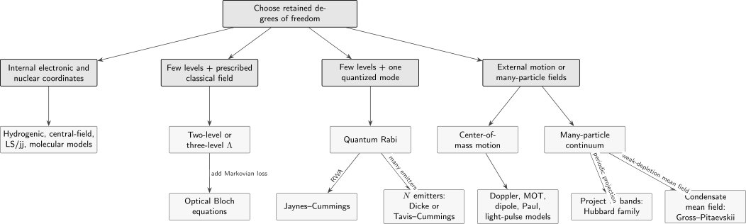
Changing the retained boundary changes the model. Quantizing a drive adds a bosonic mode; adding irreversible channels changes a Hamiltonian problem into an open-system problem; projecting motion into a band produces lattice models; replacing a dilute Bose field by its condensate amplitude produces Gross–Pitaevskii theory.

The arrows are reductions, not identities. Every arrow has a regime test. For example, Jaynes–Cummings follows from a suitable quantum Rabi Hamiltonian only when counter-rotating effects are perturbative for the observable and time scale of interest.

Quick Decision Table

Physical question	First model to inspect	Do not stop there when
bound electronic structure of a one-electron atom	hydrogenic atom	fine structure, finite mass, external fields, or core penetration resolve the Coulomb degeneracy
many-electron atom with an approximately spherical core	central-field or alkali quantum-defect model	correlation, configuration mixing, or relativistic coupling controls the observable
molecular bonding or potential curves	Born–Oppenheimer electronic model	derivative couplings, conical intersections, or nuclear quantum effects are large
one near-resonant transition under a coherent classical field	driven two-level atom	leakage, multiple Zeeman levels, spontaneous emission, or field quantization matters
driven transition with relaxation and dephasing	optical Bloch equations	the bath has memory, the drive is quantum, or more than two levels participate
one emitter and one quantized mode	quantum Rabi or Jaynes–Cummings model	multimode structure, gauge-sensitive truncation, drive, or loss matters
many equivalent emitters and one common mode	Dicke or Tavis–Cummings model	couplings are inhomogeneous or independent emission channels destroy permutation symmetry
laser threshold and mean output	rate-equation laser model	phase noise, multimode competition, spatial hole burning, or quantum fluctuations are central
near-resonant radiative force	Doppler or magneto-optical force model	sub-Doppler polarization gradients, multilevel pumping, recoil quantization, or reabsorption matters
dilute coherent Bose gas	Gross–Pitaevskii equation	depletion, fragmentation, strong correlations, or thermal kinetics is appreciable
particles in a deep optical lattice	Hubbard or Bose–Hubbard model	higher bands, long-range interactions, heating, or continuum motion is relevant
short light-pulse inertial sensor	light-pulse atom-interferometer model	finite pulse duration, wavefronts, rotations, gradients, interactions, or multilevel diffraction matter

Atomic-Structure Models

Atomic models differ mainly in how they replace or organize the electron– electron interaction and relativistic couplings.

Model	Retained structure	Decisive approximation	Canonical or nearest page
hydrogenic atom with perturbations	one electron, nuclear Coulomb field, selected correction operators	non-Coulomb terms are small relative to the gross spectrum and are treated in a declared hierarchy	Hydrogen as Atomic Prototype, Fine Structure, Hyperfine Structure, Zeeman Effect, and Stark Effect
helium variational model	two electrons in a Coulomb field	a parameterized trial space replaces the exact correlated wavefunction	Helium Atom and Variational Helium Notebook
central-field atom	independent orbitals in a spherical effective potential	nonspherical and residual correlation terms are omitted or added perturbatively	Central-Field Approximation
alkali atom with quantum defects	one valence electron plus a structured closed-shell core	core penetration and polarization are compressed into channel-dependent defects	Alkali Atoms
LS-coupled atom	total orbital $L$ and total spin $S$ are coupled before $J$	electrostatic term splittings dominate one-electron spin–orbit splittings	LS Coupling
jj-coupled atom	each $l_i$ couples to $s_i$ before the $j_i$ are combined	one-electron spin–orbit splittings dominate residual electrostatic recoupling	jj Coupling

Hydrogenic baseline

The model signature is

$$H = \frac{\mathbf p^2}{2\mu} - \frac{Ze^2}{4\pi\varepsilon_0r} + H_{\mathrm{corr}},$$

where $H_{\mathrm{corr}}$ is not one universal operator. It may include fine-structure, recoil, finite nuclear size, hyperfine, Lamb-shift, Zeeman, or Stark terms. A trustworthy calculation states which terms are included and whether degenerate perturbation theory is required.

The smallness test is matrix-element based:

$$\frac{ \left| \langle a|H_{\mathrm{corr}}|b\rangle \right| }{ \left| E_a^{(0)}-E_b^{(0)} \right| } \ll1$$

for states outside the retained degenerate or quasi-degenerate block. A small operator coefficient does not justify nondegenerate perturbation theory when the denominator is also small.

Central field, LS, and jj are a hierarchy

A central-field basis supplies one-electron orbitals. LS and jj coupling then organize angular momenta in different energy-scale limits. They are not three competing exact Hamiltonians. In intermediate coupling, neither $LSJ$ nor the set of individual $j_i$ values is exact, and configuration-interaction eigenvectors should be reported through their dominant components and mixing coefficients.

Molecular Models

The first boundary choice in molecular physics is whether nuclei are fixed, adiabatic, or fully dynamical.

Model	Retained structure	Decisive approximation	Canonical or nearest page
H₂⁺ molecular ion	one electron and two nuclei	a fixed-nuclei electronic problem is solved before nuclear motion	H₂⁺ Ion
H₂ in the Heitler–London approximation	two localized one-electron orbitals with antisymmetrized spin-space states	ionic configurations and orbital relaxation are restricted in the minimal form	Hydrogen Molecule
harmonic molecular vibration	quadratic potential in mass-weighted displacements	excursions remain near one stable minimum and mode coupling is negligible at leading order	Vibrations of Diatomics
Morse oscillator	one anharmonic dissociating coordinate	a one-dimensional empirical potential represents the selected bond coordinate	Vibrations of Diatomics
rigid rotor with centrifugal distortion	molecular orientation and a perturbative bond-stretch correction	vibrational and electronic states are fixed; rotation-induced deformation is small	Rotations of Molecules and Rotational Spectroscopy
linear-molecule normal modes	small mass-weighted nuclear displacements	the Hessian at one equilibrium geometry controls the leading motion	Normal Modes of Polyatomics

Local potential models

Near a nondegenerate minimum $R_e$, a diatomic potential has the local form

$$V(R) = V(R_e) + \frac12\mu\omega_e^2(R-R_e)^2 + O\!\left((R-R_e)^3\right).$$

The harmonic oscillator is therefore a local asymptotic model, not a global bond potential. A common Morse convention is

$$V_{\mathrm M}(R) = D_e \left[ 1-e^{-a(R-R_e)} \right]^2,$$

with the zero at the well bottom. It captures a finite dissociation energy and decreasing level spacing, but it is not an ab initio electronic-structure method and does not reproduce every long-range tail.

For a near-rigid diatomic, the leading rotational term and centrifugal distortion are commonly summarized by

$$\frac{E_J}{hc} = B_vJ(J+1) - D_v \left[ J(J+1) \right]^2 +\cdots.$$

The distortion expansion fails before arbitrarily large $J$; fitted constants must not be extrapolated past the data or past the onset of strong rovibrational mixing.

Coherent and Open Few-Level Models

Driven two-level atom

Use the Two-Level Atom when one pair of states is spectrally isolated and the applied field can be treated classically. In one rotating-frame convention,

$$H_{\mathrm{2L}} = \frac{\hbar}{2} \left( -\Delta\sigma_z + \Omega_x\sigma_x + \Omega_y\sigma_y \right).$$

This closed Hamiltonian predicts unitary Rabi dynamics. It does not by itself predict spontaneous emission, irreversible dephasing, optical pumping into unmodeled states, or photon statistics.

The truncation test is not merely “the drive is near resonance.” Off-resonant couplings to every excluded level $r$ should satisfy a scale test such as

$$\frac{|\Omega_{r}|}{|\Delta_r|} \ll1,$$

unless the associated AC Stark shift or Raman coupling is retained explicitly.

Three-level Λ system

A Λ system retains two lower states $|1\rangle$, $|2\rangle$ and one excited state $|e\rangle$. A useful rotating-frame convention is

$$\begin{aligned} \frac{H_\Lambda}{\hbar} ={}& -\Delta_p|e\rangle\langle e| -\delta|2\rangle\langle2| \\ &+ \frac12 \left( \Omega_p|e\rangle\langle1| + \Omega_c|e\rangle\langle2| + \mathrm{h.c.} \right), \end{aligned}$$

where $\delta$ is the two-photon detuning in this convention. The model is a topology, not a complete dynamics: EIT requires probe response and decoherence, while STIRAP requires time-dependent pulses and an adiabaticity test.

Use Electromagnetically Induced Transparency for the susceptibility and dark-resonance problem, and STIRAP for adiabatic population transfer. Those are the nearest canonical homes rather than duplicate Λ-model derivations.

Optical Bloch equations

The Optical Bloch Equations add a Markovian open-system contract to the driven two-level Hamiltonian. With

$$\mathcal D[L]\rho = L\rho L^\dagger - \frac12 \left\{ L^\dagger L,\rho \right\},$$

one common convention is

$$\dot\rho = -\frac{i}{\hbar}[H_{\mathrm{2L}},\rho] + \Gamma\mathcal D[\sigma_-]\rho + \frac{\gamma_\phi}{2} \mathcal D[\sigma_z]\rho.$$

Here the optical coherence decays at $\Gamma/2+\gamma_\phi$. Rate symbols vary across the literature, so this relationship is more informative than the bare symbol $\gamma$.

Optical Bloch dynamics is the right first model for saturation, power broadening, fluorescence rate, and damped Rabi oscillations. It is not a microscopic derivation of the electromagnetic reservoir, and it can fail for structured baths, strong non-Markovian feedback, multilevel optical pumping, or a quantum drive.

Quantized Light–Matter Models

Model	Retained system	Defining choice	Canonical or nearest page
quantum Rabi model	one two-level system and one bosonic mode	rotating and counter-rotating terms are retained	Rabi Model
Jaynes–Cummings model	one two-level system and one bosonic mode	the rotating-wave interaction conserves excitation number	Jaynes–Cummings Model
Dicke model	many equivalent two-level systems and one common mode	permutation-symmetric collective coupling is retained	Dicke Model
single-mode cavity	one normalized electromagnetic oscillator, optionally with ports and loss	all other modes are neglected or absorbed into calibrated rates	Quantized Electromagnetic Modes, Optical Cavities, and Cavity QED

Rabi versus Jaynes–Cummings

In a shared convention,

$$\begin{aligned} H_{\mathrm R} ={}& \hbar\omega_c a^\dagger a + \frac{\hbar\omega_a}{2}\sigma_z + \hbar g(a+a^\dagger)\sigma_x, \\ H_{\mathrm{JC}} ={}& \hbar\omega_c a^\dagger a + \frac{\hbar\omega_a}{2}\sigma_z \\ &+ \hbar g \left( a\sigma_+ + a^\dagger\sigma_- \right). \end{aligned}$$

Jaynes–Cummings removes $a\sigma_-$ and $a^\dagger\sigma_+$. Near resonance, a useful first diagnostic is

$$\frac{g\sqrt{n+1}}{\omega_a+\omega_c}\ll1$$

over the populated photon-number range. This is not a universal error bound: long evolution times, precision shifts, strong drive, high occupation, and gauge-sensitive few-level truncations require a more specific check.

The distinction from semiclassical Rabi oscillations is categorical. In the semiclassical problem, the drive amplitude is prescribed. In the quantum models, photon number is dynamical, atom and field can entangle, and vacuum fluctuations give a nonzero coupling matrix element.

Dicke and collective coupling

For $N$ equivalent emitters, define $J_\alpha=\tfrac12\sum_{j=1}^N\sigma_j^\alpha$. A common closed Dicke Hamiltonian is

$$H_{\mathrm D} = \hbar\omega_c a^\dagger a + \hbar\omega_aJ_z + \frac{2\hbar g}{\sqrt N} (a+a^\dagger)J_x.$$

The symmetric collective-spin reduction is justified only when emitter frequencies, couplings, and relevant decay channels preserve the required permutation symmetry. The equilibrium Dicke-model phase transition is also not synonymous with a transient superradiant pulse. Gauge constraints, diamagnetic terms, drive, loss, finite $N$, and multimode structure determine which laboratory interpretation is valid.

One cavity mode is a boundary choice

The ideal cavity Hamiltonian

$$H_c = \hbar\omega_c \left( a^\dagger a+\frac12 \right)$$

does not specify a laboratory resonator completely. A driven open cavity also needs port conventions, drive amplitude, detuning, and loss, often through a term $\kappa\mathcal D[a]\rho$. The one-mode model should be checked against free spectral range, polarization splitting, transverse-mode spacing, and the bandwidth of the excitation and measurement.

Optical Networks and Laser Models

Model	State variables	Primary use	Canonical page
rate-equation laser	population inversion and intracavity photon number or intensity	threshold, steady output, gain clamping, and relaxation oscillations	Rate-Equation Lasers
beam-splitter unitary	two input and two output optical modes	interference, Fock-state transformations, and lossless mode mixing	Beam Splitters
Mach–Zehnder interferometer	two beam splitters plus relative propagation phase	phase-to-count or phase-to-intensity transduction	Interferometers

Rate-equation laser

A minimal class-B-style structure is

$$\begin{aligned} \dot N &= R_p - \frac{N}{\tau} - G(N)S, \\ \dot S &= \Gamma_cG(N)S + \beta\frac{N}{\tau} - \frac{S}{\tau_p}. \end{aligned}$$

$N$, $S$, the confinement factor $\Gamma_c$, and the gain convention must be defined before comparing formulas. These equations average over optical phase and often over space. They are not the right endpoint for Schawlow–Townes linewidth, quantum intensity noise, mode locking, spatial hole burning, or coherent transients.

Beam splitter and Mach–Zehnder

A lossless two-port beam splitter is a $U(2)$ mode transformation. One common phase convention is

$$\begin{pmatrix} a_{\mathrm{out}}\\ b_{\mathrm{out}} \end{pmatrix} = \begin{pmatrix} t & r\\ -r^* & t^* \end{pmatrix} \begin{pmatrix} a_{\mathrm{in}}\\ b_{\mathrm{in}} \end{pmatrix}, \qquad |t|^2+|r|^2=1.$$

Different sign and phase conventions describe the same device when used consistently. A Mach–Zehnder model composes two such transformations with a relative phase. Loss, detector POVMs, mode mismatch, and partial distinguishability are separate physical ingredients, not alternative beam- splitter conventions.

Cooling, Trapping, and Control Models

Model	Leading reduced law	Use when	Canonical page
Doppler cooling force	velocity-dependent radiation-pressure imbalance	a near-two-level particle samples counterpropagating red-detuned beams	Doppler Cooling
magneto-optical trap	damping plus position-dependent restoring force	Zeeman shifts and polarized beams create a stable linearized trap	Magneto-Optical Traps
optical dipole trap	conservative dynamic-polarizability potential plus scattering	light is sufficiently far detuned that internal excitation can be eliminated	Optical Dipole Traps
Paul-trap secular motion	harmonic pseudopotential with micromotion corrections	Mathieu parameters lie in a stable region and time-scale separation is adequate	Ion Traps
Rydberg blockade model	driven two-level sites with strong state-dependent pair shifts	an interaction shift resolves or suppresses multiple Rydberg excitation	Rydberg Blockade
light-pulse atom interferometer	internal-state-dependent momentum kicks and free propagation	short coherent pulses act as matter-wave beam splitters and mirrors	Atom Interferometry

Linearized force models

For two counterpropagating beams, the one-dimensional Doppler force has the structure

$$F(v) = \hbar k \left[ R_+(v)-R_-(v) \right] \simeq -\alpha v$$

near $v=0$. A one-dimensional magneto-optical trap adds a linear restoring term,

$$F(x,v) \simeq -\kappa_xx-\alpha v.$$

These are local expansions. Capture velocity, beam profile, optical pumping, magnetic-field geometry, diffusion, and gravity can all invalidate a global harmonic interpretation.

For a far-detuned field, an optical dipole potential can be written in terms of the dynamic polarizability as

$$U(\mathbf r) = -\frac14 \operatorname{Re}\alpha(\omega) |\mathbf E_0(\mathbf r)|^2$$

for a complex-amplitude convention $\mathbf E(t)=\operatorname{Re}[\mathbf E_0e^{-i\omega t}]$. The associated photon-scattering rate must be checked independently; “conservative” is an approximation, not a property of all optical traps.

Paul trap

Each ideal quadrupole coordinate reduces to a Mathieu equation,

$$\frac{d^2u}{d\tau^2} + \left[ a_u-2q_u\cos(2\tau) \right]u =0.$$

The secular pseudopotential averages over radio-frequency micromotion. It should not be used to erase excess micromotion, nonlinear fields, parametric resonances, or motion outside the stability region.

Rydberg blockade

A common frozen-position model is

$$\begin{aligned} \frac{H}{\hbar} ={}& \frac{\Omega}{2}\sum_i\sigma_i^x - \Delta\sum_i n_i \\ &+ \sum_{i<j} \frac{V_{ij}}{\hbar} n_in_j, \end{aligned}$$

where $n_i=|r_i\rangle\langle r_i|$. “Perfect blockade” means that relevant interaction shifts are large compared with the excitation linewidth and coupling scale; finite blockade, anisotropy, motion, decay, and unwanted pair resonances require the full calibrated interaction.

Light-pulse atom interferometer

For an ideal three-pulse Mach–Zehnder sequence in a uniform acceleration, the leading inertial phase is

$$\Phi_a = \mathbf k_{\mathrm{eff}}\cdot\mathbf a\,T^2$$

up to the chosen laser-phase and sign conventions. This compact model assumes short pulses, a specified momentum-transfer order, controlled trajectories, and a uniform acceleration. Precision sensors must add finite-pulse response, laser phase noise, wavefront curvature, gravity gradients, rotations, velocity distributions, and detection systematics.

Lattice and Condensate Models

Optical-lattice Hubbard model

The optical-lattice page owns the continuum-to-lattice experimental reduction; the many-body volume owns the canonical Hubbard Hamiltonian. For spin-$1/2$ fermions,

$$\begin{aligned} H ={}& -t \sum_{\langle i,j\rangle,\sigma} \left( c_{i\sigma}^\dagger c_{j\sigma} + \mathrm{h.c.} \right) \\ &+ U\sum_i n_{i\uparrow}n_{i\downarrow}. \end{aligned}$$

Use Optical Lattices for band formation, Wannier functions, recoil scales, loading, and calibration. Use the Hubbard Model for the canonical fermionic model, and the Bose–Hubbard Model for lattice bosons.

A single-band reduction requires the retained energy scales, including $t$, $U$, $k_{\mathrm B}T$, drive bandwidth, and interaction-induced band mixing, to remain controlled relative to relevant interband gaps. Long-range interactions, density-assisted hopping, and heating are physical corrections, not numerical noise.

Gross–Pitaevskii equation

For a dilute, weakly depleted Bose condensate, the number-normalized field $\Psi$ obeys

$$i\hbar\partial_t\Psi = \left[ -\frac{\hbar^2\nabla^2}{2m} + V_{\mathrm{ext}} + g|\Psi|^2 \right]\Psi, \qquad \int d^3r\,|\Psi|^2=N.$$

In three dimensions at leading low energy,

$$g = \frac{4\pi\hbar^2a_s}{m}.$$

The canonical derivation and validity analysis live in the Gross–Pitaevskii Equation. The Bose–Einstein Condensates Overview connects it to AMO preparation and diagnostics.

The local dilute-gas parameter

$$n|a_s|^3\ll1$$

is necessary but not by itself sufficient. The condensate fraction, thermal component, dimensional reduction, loss, fragmentation, and dynamical instabilities must also match the chosen equation.

Hubbard versus Gross–Pitaevskii

These models are not selected by whether the particles are “cold.” Choose a lattice model when discrete Wannier orbitals and site occupations are the retained variables. Choose Gross–Pitaevskii theory when a coherent continuum condensate field is the retained variable and correlations beyond mean field are small. A condensate in a shallow lattice can require a Gross–Pitaevskii equation with a periodic potential; a deep lattice near a number-correlated regime can require Bose–Hubbard dynamics.

Controlled Relations Between Models

Starting description	Reduction	Result	Required check
multilevel atom plus classical field	spectrally isolate two states and eliminate the rest	driven two-level model	leakage and induced shifts from excluded states
closed driven two-level model	add calibrated Markovian decay and dephasing	optical Bloch equations	bath correlation time and closure of the two-level manifold
Λ Hamiltonian	large one-photon detuning and adiabatic elimination	effective Raman two-level model	excited-state population and spontaneous-scattering error
quantum Rabi model	rotating-wave approximation	Jaynes–Cummings model	counter-rotating corrections across populated manifolds and times
$N$ equivalent Rabi couplings	collective-spin restriction	Dicke model	permutation symmetry and inhomogeneity
continuum particles in a periodic potential	project into localized Wannier orbitals	Hubbard-family model	band gap, interaction-induced mixing, and omitted matrix elements
dilute interacting Bose field	replace the field operator by a condensate amplitude	Gross–Pitaevskii equation	depletion, gas parameter, and fluctuation observables
Mathieu ion motion	average over the radio-frequency period	secular pseudopotential	stability parameters and micromotion sensitivity
full molecular potential near one minimum	quadratic expansion and normal-mode rotation	harmonic vibrational model	displacement amplitude, resonances, and anharmonic residuals

An effective model should inherit an error budget. If a reduction introduces small parameters $\epsilon_1,\epsilon_2,\ldots$, a useful validation report does not merely list them; it compares observables at successive model levels,

$$\delta_O = \frac{ \left| O_{\mathrm{reduced}} - O_{\mathrm{parent}} \right| }{ O_{\mathrm{scale}} },$$

over the actual parameter region and time interval.

Common Model-Selection Mistakes

Choosing by visual resemblance

Damped oscillations do not uniquely imply optical Bloch equations. They can come from ensemble dephasing, leakage, technical noise, non-Markovian memory, or unresolved coherent frequencies. Identify the retained variables and test residuals.

Calling every two-state equation the Rabi model

A prescribed classical drive, a quantized single mode, and a rotating-wave quantized mode correspond to the driven two-level, quantum Rabi, and Jaynes–Cummings models, respectively.

Adding a linewidth without changing the model

Replacing $\omega$ by a complex number can reproduce a line shape in a limited calculation, but it does not automatically define a completely positive density-operator evolution or the associated noise.

Treating a basis truncation as a physical approximation

Keeping ten cavity Fock states is a numerical cutoff. Keeping one cavity mode is a physical model reduction. Both require convergence or validity tests, but their errors have different meanings.

Extrapolating local models globally

Harmonic potentials, linear MOT forces, secular Paul-trap motion, and single-band Hubbard parameters are local or scale-separated descriptions. They should not be extrapolated into dissociation, capture, instability, or interband regimes without revalidation.

Ignoring conventions in a familiar Hamiltonian

Factors of two can move among Rabi frequency, Pauli operators, collective couplings, field amplitudes, and Lindblad rates. Compare a measurable splitting, decay rate, or transfer probability rather than matching symbols.

Model-Choice Exercises

Exercise 1: Classical drive, Rabi, or Jaynes–Cummings?

An atom is driven by a laser whose depletion and photon-number fluctuations are negligible. A calculation is needed for coherent population transfer over ten Rabi periods. Which model should be the baseline?

Solution

Use the driven two-level Hamiltonian if leakage to other atomic levels and decoherence are negligible over the ten-period interval. The quantum Rabi and Jaynes–Cummings models make the field mode dynamical, which is unnecessary when the laser is accurately prescribed as a classical field. Add optical Bloch terms if measured decay or dephasing is relevant.

Exercise 2: Testing the rotating-wave approximation

A cavity experiment has $\omega_a\simeq\omega_c$, coupling $g$, and appreciable population through photon number $n_{\max}$. State a first diagnostic for choosing Jaynes–Cummings over the quantum Rabi model.

Solution

Check that

$$\frac{g\sqrt{n_{\max}+1}}{\omega_a+\omega_c}\ll1.$$

Then compare the observable of interest against the parent Rabi model over the actual evolution time. Precision shifts or long-time phases can reveal small counter-rotating corrections even when short-time populations look accurate.

Exercise 3: One Λ system, two questions

The same three levels are used first to measure a narrow transparency window and later to transfer population with counterintuitive pulses. Which canonical homes apply?

Solution

Use Electromagnetically Induced Transparency for probe susceptibility, absorption, dispersion, and decoherence. Use STIRAP for time-dependent dark-state following, pulse order, and adiabatic transfer. The level topology is the same, but the observables and validity tests differ.

Exercise 4: Harmonic or Morse?

Measured vibrational spacings decrease steadily with excitation and states approach a dissociation threshold. Why is a harmonic model structurally insufficient, and what is a useful next model?

Solution

A harmonic oscillator has equally spaced levels and no finite dissociation energy. A Morse oscillator is a useful one-coordinate next model because it has a finite asymptote and decreasing bound-state spacing. It remains an effective potential and should be checked against the measured or computed potential curve, especially near long range.

Exercise 5: Continuum condensate or lattice occupations?

Bosons occupy a deep optical lattice near unit filling, and number fluctuations are strongly suppressed. Should a single coherent Gross–Pitaevskii field be the default?

Solution

No. The retained observables are site occupations and their correlations, and strong number squeezing signals physics beyond a single coherent mean field. A Bose–Hubbard model is the natural baseline, after validating the single-band projection. Gross–Pitaevskii theory may still describe a shallow- lattice superfluid regime, but it is not selected merely because the particles are bosons.

Exercise 6: Secular motion and micromotion

An ion’s slow oscillation frequency is predicted accurately by a Paul-trap pseudopotential, but a clock shift depends on radio-frequency kinetic energy. Is the secular model sufficient?

Solution

Not by itself. The pseudopotential can predict the slow secular frequency while averaging away intrinsic and excess micromotion. A clock-shift calculation sensitive to radio-frequency kinetic energy must restore micromotion using the Mathieu solution or an equivalently validated time-dependent model.

Exercise 7: Closed cavity exchange with loss

One emitter swaps an excitation with one cavity mode while photons leak through a mirror. Which model owns each part?

Solution

The Jaynes–Cummings Hamiltonian owns the coherent rotating-wave exchange. Cavity QED supplies the physical coupling and linewidth regime, while a quantum optical master equation adds cavity loss and emitter decay. Calling the entire open problem “Jaynes–Cummings” without naming the dissipators leaves the dynamics underspecified.

Exercise 8: A hierarchy, not a winner

An atom has electrostatic term splittings and one-electron spin–orbit splittings of comparable size. Should its states be labeled by pure LS or pure jj coupling?

Solution

Neither limit is exact. Diagonalize the relevant Hamiltonian in a suitable configuration basis and report intermediate-coupling eigenvectors through their dominant LS- or jj-coupled components. The limiting schemes remain useful bases and diagnostics, not exact quantum numbers.

Cross-Links

• Reference and Data is the task-oriented gateway to AMO lookup pages and source-provenance rules.
• Common Atomic Hamiltonians compares the operator content, units, symmetries, and regime tests of the standard atomic models indexed here.
• Atomic, Molecular, and Optical Physics
• Atomic Physics
• Molecular Quantum Mechanics
• Light–Matter Interaction
• Quantum Optics
• AMO Platforms and Control
• Computational AMO and Quantum Chemistry
• Reference Model Encyclopedia
• Choosing a Method
• Common Many-Body Hamiltonians
• Approximation Checklist

References

• H. A. Bethe and E. E. Salpeter, Quantum Mechanics of One- and Two-Electron Atoms, Springer, 1957.
• R. N. Zare, Angular Momentum: Understanding Spatial Aspects in Chemistry and Physics, Wiley, 1988.
• G. Herzberg, Molecular Spectra and Molecular Structure I: Spectra of Diatomic Molecules, 2nd ed., Van Nostrand, 1950.
• P. F. Bernath, Spectra of Atoms and Molecules, 4th ed., Oxford University Press, 2020.
• C. Cohen-Tannoudji, J. Dupont-Roc, and G. Grynberg, Atom–Photon Interactions: Basic Processes and Applications, Wiley, 1992.
• L. Allen and J. H. Eberly, Optical Resonance and Two-Level Atoms, Dover, 1987.
• E. T. Jaynes and F. W. Cummings, “Comparison of Quantum and Semiclassical Radiation Theories with Application to the Beam Maser”, Proceedings of the IEEE 51, 89–109, 1963.
• I. I. Rabi, “On the Process of Space Quantization”, Physical Review 49, 324–328, 1936.
• R. H. Dicke, “Coherence in Spontaneous Radiation Processes”, Physical Review 93, 99–110, 1954.
• J. Hubbard, “Electron Correlations in Narrow Energy Bands”, Proceedings of the Royal Society A 276, 238–257, 1963.
• E. P. Gross, “Structure of a Quantized Vortex in Boson Systems”, Il Nuovo Cimento 20, 454–477, 1961.
• L. P. Pitaevskii, “Vortex Lines in an Imperfect Bose Gas”, Soviet Physics JETP 13, 451–454, 1961.
• E. L. Raab, M. Prentiss, A. Cable, S. Chu, and D. E. Pritchard, “Trapping of Neutral Sodium Atoms with Radiation Pressure”, Physical Review Letters 59, 2631–2634, 1987.
• W. Paul, “Electromagnetic Traps for Charged and Neutral Particles”, Reviews of Modern Physics 62, 531–540, 1990.
• M. Kasevich and S. Chu, “Atomic Interferometry Using Stimulated Raman Transitions”, Physical Review Letters 67, 181–184, 1991.