Bose–Einstein Condensates Overview

A Bose–Einstein condensate is a many-boson state with macroscopic occupation of one one-particle natural orbital. In dilute atomic gases, that mode can often be represented by a complex field whose density and phase obey the Gross–Pitaevskii equation. The definition is spectral and many-body; the field equation is an approximation; and an experimental claim is an inference from calibrated observables. Keeping those three levels separate is the central discipline of condensate physics.

This page is an AMO-facing guide to that chain:

$$\begin{gathered} \text{macroscopic natural occupation} \longrightarrow \text{effective field} \longrightarrow \text{predicted density and dynamics}, \\ \text{prepared cloud} \longrightarrow \text{images, correlations, and response} \longrightarrow \text{model-tested condensate claim}. \end{gathered}$$

The phrase “all atoms occupy the same wavefunction” is useful only as a first idealization. A real gas can contain a thermal component, quantum depletion, several internal states, vortices, fragmented occupations, and finite-size phase fluctuations. A trustworthy analysis therefore reports which mode is macroscopically occupied, which effective theory is being used, and which measurements constrain its assumptions.

Canonical Scope

This page owns:

1. the AMO interpretation of macroscopic occupation in a trapped gas;
2. the relation between a condensate natural orbital and a complex order parameter;
3. a working overview of the Gross–Pitaevskii equation and its validity ledger;
4. collective modes, expansion, interference, and coherence as laboratory diagnostics;
5. a workflow for supporting a condensate claim with complementary observables.

The full equilibrium criterion, ideal-gas transition, dimensionality, and condensate-fraction formulas live in Bose–Einstein Condensation. Off-Diagonal Long-Range Order owns the reduced-density-matrix hierarchy and thermodynamic-limit statements. Gross–Pitaevskii Equation owns the full variational derivation, normalization conventions, hydrodynamics, vortices, and stability analysis. Bogoliubov Theory owns the quadratic fluctuation theory and its canonical diagonalization.

Here those results are used as a compact bridge from laboratory controls to observable behavior.

Macroscopic Occupation

The basis-independent definition

For a bosonic field operator $\hat\psi(\mathbf r)$, define the one-body density matrix

$$\rho^{(1)}(\mathbf r,\mathbf r') = \left\langle \hat\psi^\dagger(\mathbf r') \hat\psi(\mathbf r) \right\rangle.$$

It is a positive Hermitian kernel with

$$\int d^3r\, \rho^{(1)}(\mathbf r,\mathbf r) = N.$$

Its spectral decomposition is

$$\rho^{(1)}(\mathbf r,\mathbf r') = \sum_\alpha N_\alpha \phi_\alpha(\mathbf r) \phi_\alpha^*(\mathbf r'),$$

where the orthonormal $\phi_\alpha$ are natural orbitals and the $N_\alpha$ are their occupations. Bose–Einstein condensation occurs when, in the relevant large-system limit,

$$N_0 = O(N).$$

For a simple condensate, one eigenvalue is extensive and the others are subextensive. If several eigenvalues are extensive, the condensate is fragmented. A large occupation in an arbitrarily chosen basis is not the criterion; diagonalizing $\rho^{(1)}$ identifies the physically distinguished modes.

The condensate fraction is

$$f_0 = \frac{N_0}{N}.$$

It is neither the thermal ground-state population in every basis nor the superfluid fraction. The latter is a response coefficient, inferred for example from phase stiffness, nondissipative flow, or rotational response. The two quantities can differ substantially.

Why the trap ground state is not always the condensate orbital

For an ideal gas in a static trap, the most occupied natural orbital below the transition is the one-particle trap ground state. Interactions deform that orbital. Repulsive interactions broaden it; attraction narrows it and can eventually destabilize the cloud; rotation can produce a vortex texture; multicomponent couplings can produce spinor or fragmented structure.

Thus “ground state” must be qualified:

• one-particle trap ground state refers to the eigenstate of $-\hbar^2\nabla^2/(2m)+V$;
• condensate orbital refers to the leading eigenvector of $\rho^{(1)}$;
• many-body ground state refers to the lowest eigenstate of the full interacting Hamiltonian;
• stationary mean-field state is a critical point of an approximate energy functional.

They coincide only under additional assumptions.

A trapped ideal-gas benchmark

For $N\gg1$ noninteracting bosons in a three-dimensional harmonic trap with geometric-mean angular frequency

$$\bar\omega = \left( \omega_x\omega_y\omega_z \right)^{1/3},$$

the semiclassical transition scale is

$$k_{\mathrm B}T_c^{(0)} = \hbar\bar\omega \left[ \frac{N}{\zeta(3)} \right]^{1/3}.$$

Below this scale, the leading ideal result is

$$\frac{N_0}{N} \simeq 1- \left( \frac{T}{T_c^{(0)}} \right)^3.$$

For $N=10^5$ and $\bar\omega/(2\pi)=100\ \mathrm{Hz}$,

$$T_c^{(0)} \simeq 2.10\times10^{-7}\ \mathrm K = 210\ \mathrm{nK}.$$

This estimate is a scale setter, not a fit formula valid without qualification. Finite-size corrections, interactions, anharmonicity, internal-state mixtures, and imperfect equilibrium all shift the observed crossover. In a finite trap there is no literal thermodynamic singularity; one observes a rapidly growing leading occupation over a finite temperature interval.

From a Mode to an Effective Field

Number-normalized order parameter

When one natural orbital dominates and depletion is modest, define

$$\Psi(\mathbf r,t) = \sqrt{N_0}\, \phi_0(\mathbf r,t) = \sqrt{n_0(\mathbf r,t)} e^{i\theta(\mathbf r,t)}$$

with

$$\int d^3r\, \lvert\Psi(\mathbf r,t)\rvert^2 = N_0.$$

Then $n_0=\lvert\Psi\rvert^2$ is condensate number density. It is not a one-particle probability density. A common alternative normalizes the orbital to one and writes $\Psi=\sqrt{N_0}\phi_0$; mixing these conventions without moving the factor of $N_0$ is a frequent source of wrong nonlinearities.

Writing $\Psi=\sqrt{n_0}e^{i\theta}$ makes the kinematics transparent. The mean-field current and velocity are

$$\begin{aligned} \mathbf j &= \frac{\hbar}{m} \operatorname{Im} \left( \Psi^*\nabla\Psi \right), \\ \mathbf v &= \frac{\mathbf j}{n_0} = \frac{\hbar}{m} \nabla\theta \end{aligned}$$

wherever $n_0\neq0$. Single-valuedness gives quantized circulation around a closed contour that does not cross a node:

$$\oint\mathbf v\cdot d\boldsymbol\ell = \frac{h}{m}\,\ell, \qquad \ell\in\mathbb Z.$$

This connects phase topology to quantized vortices, but vortex observation is a superfluid-response diagnostic in addition to being compatible with condensation.

The fixed-number caveat

In an exact state with sharp total particle number,

$$\left\langle \hat\psi(\mathbf r) \right\rangle = 0$$

because $\hat\psi$ changes the number sector. The same state can still have an extensive eigenvalue of $\rho^{(1)}$. Therefore $\Psi=\langle\hat\psi\rangle$ is not a universal microscopic definition of condensation.

The complex field can instead be understood as:

• a symmetry-broken representative in the thermodynamic limit;
• a number-conserving condensate orbital multiplied by $\sqrt{N_0}$;
• a relative-phase field defined with respect to another condensate, local oscillator, or measurement record.

A global phase is not observable. Phase differences, currents, interference fringes, and correlation functions are observable.

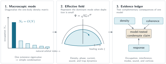
A condensate claim connects three levels. A dominant eigenvalue $N_0$ defines macroscopic occupation; a controlled approximation represents that mode by $\Psi=\sqrt{n_0}e^{i\theta}$; complementary density, coherence, and response measurements test the representation and its physical interpretation.

Gross–Pitaevskii Equation Overview

Contact-interaction model

For one dilute condensate component in three dimensions, with short-range $s$-wave interactions and scattering length $a$, the leading coupling is

$$g = \frac{4\pi\hbar^2a}{m}.$$

The number-normalized Gross–Pitaevskii energy functional is

$$\begin{aligned} E[\Psi] = \int d^3r\, \bigg[ & \frac{\hbar^2}{2m} \lvert\nabla\Psi\rvert^2 + V(\mathbf r) \lvert\Psi\rvert^2 \\ & + \frac{g}{2} \lvert\Psi\rvert^4 \bigg]. \end{aligned}$$

Its closed-system time evolution is

$$i\hbar \frac{\partial\Psi}{\partial t} = \left[ - \frac{\hbar^2\nabla^2}{2m} + V(\mathbf r,t) + g\lvert\Psi\rvert^2 \right] \Psi.$$

For a stationary solution

$$\Psi(\mathbf r,t) = e^{-i\mu t/\hbar} \psi_0(\mathbf r),$$

the equation becomes

$$\mu\psi_0 = \left[ - \frac{\hbar^2\nabla^2}{2m} + V + g\lvert\psi_0\rvert^2 \right] \psi_0.$$

The chemical potential $\mu$ enforces fixed condensate number in the stationary variational problem. It is not generally equal to $E/N_0$ because interaction pairs contribute differently to $E$ and $\mu$.

What the approximation assumes

The equation is reliable when the observable of interest is insensitive to the omitted degrees of freedom and the following ledger is favorable:

Requirement	Useful diagnostic	Failure sign
three-dimensional dilute gas	$n a^3\ll1$	strong quantum depletion or nonuniversal short-range physics
one dominant condensate mode	$N_0/N$ large and unfragmented	several extensive natural occupations
low thermal fraction	thermal density and damping are small	substantial condensate–thermal-cloud exchange
contact interaction	collision energy and range are low	effective-range, dipolar, or multichannel effects
slow coarse-grained dynamics	scales longer than microscopic collision time	violent quenches or molecular production
closed conservative evolution	loss and heating times are long	appreciable damping, recombination, or noise

The small gas parameter controls weak-coupling corrections in a stable, repulsive, homogeneous gas. It does not guarantee that every process is slow: three-body recombination, technical noise, or a rapid control ramp can still invalidate a conservative single-field model.

Near a Feshbach resonance, replacing all interaction physics by a very large $g$ is generally unsafe. Unitarity, effective range, loss, molecule formation, and depletion enter before a naive contact mean field becomes arbitrarily strong. Ultracold Atoms gives the corresponding resonance and timescale audit.

Healing length and sound speed

For a uniform repulsive gas of density $n_0$, the mean-field chemical potential is

$$\mu = gn_0.$$

Balancing kinetic and interaction energies defines the healing length

$$\xi = \frac{\hbar}{\sqrt{2mgn_0}}$$

and long-wavelength density disturbances propagate with sound speed

$$c = \sqrt{\frac{gn_0}{m}}.$$

The two scales obey

$$\xi = \frac{\hbar}{\sqrt{2}\,mc}.$$

The healing length controls how rapidly the field can recover from a hard boundary, density defect, or vortex core. It is not automatically the interparticle spacing or the thermal de Broglie wavelength.

For rubidium-87 with $a=100a_0$ and $n_0=10^{20}\ \mathrm{m^{-3}}$,

$$\begin{aligned} \frac{\mu}{h} &\simeq 773\ \mathrm{Hz}, & \frac{\mu}{k_{\mathrm B}} &\simeq 37.1\ \mathrm{nK}, \\ \xi &\simeq 0.274\ \mu\mathrm m, & c &\simeq 1.88\ \mathrm{mm\,s^{-1}}. \end{aligned}$$

These numbers provide an immediate consistency check. Imaging cannot resolve a bare vortex core if its point-spread function is much broader than $\xi$, and a ramp across a cloud of size $R$ is not globally adiabatic if it is fast compared with a sound-crossing time $R/c$.

Thomas–Fermi regime

In a repulsive condensate whose interaction energy dominates the kinetic energy over most of the cloud, the stationary density is approximately

$$n_{\mathrm{TF}}(\mathbf r) = \frac{ \mu-V(\mathbf r) }{g} \, \Theta\!\left( \mu-V(\mathbf r) \right).$$

For a harmonic trap

$$V(\mathbf r) = \frac{m}{2} \left( \omega_x^2x^2 + \omega_y^2y^2 + \omega_z^2z^2 \right),$$

the Thomas–Fermi radii satisfy

$$R_i = \sqrt{ \frac{2\mu}{m\omega_i^2} }.$$

The approximation is controlled in the bulk when the cloud dimensions are large compared with the healing length. It necessarily fails in a boundary layer near the sharp Thomas–Fermi edge and at vortex cores, where the kinetic term smooths the density. The complete derivation and normalization formula belong to Gross–Pitaevskii Equation.

Collective Modes

Uniform excitations

Linearizing about a uniform weakly interacting condensate gives the Bogoliubov dispersion

$$E_k = \sqrt{ \epsilon_k \left( \epsilon_k+2gn_0 \right) }, \qquad \epsilon_k = \frac{\hbar^2k^2}{2m}.$$

At $k\xi\ll1$,

$$E_k \simeq \hbar ck,$$

so the excitation is a collective sound wave. At $k\xi\gg1$,

$$E_k \simeq \epsilon_k+gn_0,$$

and it becomes particle-like. The crossover is physical evidence of interaction-generated rigidity, but extracting it requires a calibrated probe such as Bragg spectroscopy and a model of inhomogeneous broadening.

This dispersion is quoted here for scale interpretation. Its derivation, quasiparticle amplitudes, depletion, zero modes, and stability conditions belong to Bogoliubov Theory.

Modes in a harmonic trap

Confinement discretizes the collective spectrum. In the hydrodynamic Thomas–Fermi limit, low-order modes can often be interpreted as polynomial density and velocity fields:

Mode	Dominant motion	Ideal benchmark in an isotropic trap
dipole	center of mass	$\omega_{\mathrm d}=\omega$
quadrupole surface mode	shape oscillation at nearly fixed volume	$\omega_{\mathrm q}=\sqrt{2}\,\omega$
monopole breathing mode	radial compression and expansion	$\omega_{\mathrm b}=\sqrt{5}\,\omega$

The dipole result is unusually robust. For particles with translationally invariant interactions in a harmonic trap, center-of-mass motion separates and oscillates at the trap frequency. An interaction-dependent dipole shift therefore points first to anharmonicity, trap calibration, internal forces, or a broken assumption, not to a new equation of state.

The quadrupole and breathing frequencies depend on geometry, collisional regime, dimensionality, and equation of state. Their damping can reflect Landau or Beliaev processes, thermal-cloud collisions, dephasing from anharmonicity, or technical noise. A fitted damped sinusoid does not by itself identify the microscopic damping channel.

Hydrodynamic interpretation

With $\Psi=\sqrt n e^{i\theta}$, the Gross–Pitaevskii equation separates into

$$\frac{\partial n}{\partial t} + \nabla\cdot \left( n\mathbf v \right) = 0$$

and

$$m \left[ \frac{\partial\mathbf v}{\partial t} + \left( \mathbf v\cdot\nabla \right) \mathbf v \right] = - \nabla \left[ V+gn - \frac{\hbar^2}{2m} \frac{\nabla^2\sqrt n}{\sqrt n} \right].$$

The final term is quantum pressure. It is negligible for smooth Thomas–Fermi motion but essential near edges, defects, and structures on the scale of $\xi$. Dropping it is therefore a scale-dependent approximation, not an identity.

A mode-measurement audit

A useful collective-mode report includes:

1. the trap frequencies and measured anharmonicity;
2. the excitation protocol and perturbation amplitude;
3. the equilibrium density, atom number, and interaction setting;
4. the fitted frequency, damping rate, and phase with uncertainties;
5. checks for nonlinear frequency shifts as the drive is reduced;
6. a finite-temperature or collision-regime estimate;
7. comparison with both an interaction-sensitive mode and the dipole calibration mode.

Collective response is strongest as evidence when it tests a parameter already inferred from equilibrium measurements rather than introducing a new unconstrained fit for every mode.

Expansion and Density Profiles

Bimodality

After release, a partly condensed weakly interacting gas often shows a narrow condensate component superposed on a broad thermal distribution. This bimodal structure was central to the first dilute-gas observations. It is persuasive when:

• the thermal wings are fitted in a regime where the assumed distribution is valid;
• the narrow component grows systematically below a reproducible temperature or phase-space-density scale;
• optical depth, saturation, finite resolution, and interactions during expansion are included;
• alternative nonthermal preparation mechanisms are excluded.

A two-component fit is a model comparison, not a direct diagonalization of $\rho^{(1)}$. Report residuals and compare plausible line shapes rather than treating the fit label as the conclusion.

Ballistic and hydrodynamic expansion

For a sufficiently dilute thermal gas, long time of flight approximately maps initial momentum to position,

$$\mathbf r \simeq \frac{\mathbf p}{m}\,t.$$

A condensate can expand nonballistically because mean-field interaction energy is converted into kinetic energy. In the Thomas–Fermi scaling solution, radii evolve as

$$R_i(t) = b_i(t)R_i(0),$$

where, after suddenly removing a harmonic trap,

$$\ddot b_i = \frac{\omega_i^2}{ b_i b_xb_yb_z }, \qquad b_i(0)=1, \qquad \dot b_i(0)=0.$$

A tightly confined direction initially has a larger pressure gradient and expands more rapidly. The cloud can therefore invert its aspect ratio. This anisotropic release is a strong consistency check for an interacting condensate, but it is not a unique definition: collisional thermal gases and hydrodynamic Fermi gases can also expand anisotropically.

Interference and Coherence

First-order coherence

The normalized first-order correlation function is

$$g^{(1)}(\mathbf r,\mathbf r') = \frac{ \rho^{(1)}(\mathbf r,\mathbf r') }{ \sqrt{ n(\mathbf r)n(\mathbf r') } }.$$

It measures the visibility available to a one-body interference experiment, after accounting for density. For a perfectly coherent simple condensate in the idealized rank-one limit,

$$\rho^{(1)}(\mathbf r,\mathbf r') = N_0 \phi_0(\mathbf r) \phi_0^*(\mathbf r'),$$

and the condensate contribution factorizes. Thermal occupation, phase fluctuations, multimode structure, and averaging reduce measured coherence.

In an infinite homogeneous three-dimensional condensate, a nonzero large-separation limit of the one-body kernel is one-body off-diagonal long-range order. In finite traps, “long range” is necessarily operational: one compares separations with cloud size, healing length, thermal wavelength, and phase-correlation length. In one and two dimensions, infrared phase fluctuations can replace true long-range order by algebraic or finite-size coherence.

Two expanding condensates

Suppose two initially separated modes overlap after release:

$$\Psi(\mathbf r,t) = \Psi_1(\mathbf r,t) + e^{i\varphi} \Psi_2(\mathbf r,t).$$

The density is

$$\begin{aligned} n(\mathbf r,t) = & \lvert\Psi_1\rvert^2 + \lvert\Psi_2\rvert^2 \\ & + 2\operatorname{Re} \left[ e^{i\varphi} \Psi_1^*\Psi_2 \right]. \end{aligned}$$

For sources separated by $\mathbf d$ and observed after a long expansion time $t$, the far-field fringe wavevector is approximately

$$\mathbf q \simeq \frac{m\mathbf d}{\hbar t},$$

so the fringe spacing along the separation axis is

$$\lambda_{\mathrm{fr}} \simeq \frac{ht}{md}.$$

Independent condensates need not share a reproducible phase before measurement. A single image can show high-contrast fringes with a phase that varies randomly from shot to shot. The measurement establishes a relative phase in that realization; ensemble averaging without phase alignment can erase the fringes.

What visibility does and does not establish

For local intensities $I_1$ and $I_2$ and mutual degree of coherence $\gamma_{12}$, ideal fringe visibility is

$$\mathcal V = \frac{ 2\sqrt{I_1I_2} }{ I_1+I_2 } \lvert\gamma_{12}\rvert.$$

Low visibility can result from unequal populations, phase noise, imaging resolution, integration along the line of sight, wavefront curvature, or multimode occupation. Conversely, high visibility over one baseline does not reconstruct the full one-body density matrix or prove thermodynamic off-diagonal long-range order. A coherence claim should specify baseline, averaging procedure, phase registration, and transfer function.

Coherent state is a different term

A Glauber coherent state is an eigenstate of an annihilation operator and has number fluctuations. A number-fixed condensate can have a macroscopically occupied natural orbital while not being a Glauber coherent state. “Condensate,” “phase coherent,” and “coherent state” are related but not interchangeable labels.

What Experiments Actually Establish

No single common observable is a complete definition in a finite, interacting, imperfectly measured system. Complementary probes constrain different links in the inference:

Observable	Supports	Important alternatives or nuisance parameters
bimodal density profile	rapidly growing low-momentum component	fit model, resolution, nonequilibrium tails
condensate-fraction trend	occupation transfer below a crossover	thermometry and finite-size corrections
anisotropic expansion	interaction pressure and coherent hydrodynamics	collisional normal-gas hydrodynamics
interference fringes	first-order coherence on a stated baseline	phase registration and imaging transfer
collective frequencies	equation of state and mean-field stiffness	anharmonicity and finite temperature
sound propagation	compressibility and hydrodynamic response	damping and inhomogeneous averaging
quantized vortices	phase winding and superfluid rotational response	nucleation and imaging selection
natural-orbital reconstruction	direct occupation spectrum	incomplete tomography and regularization

The most persuasive evidence is overconstrained: one set of calibrated parameters predicts several measurements. For example, atom number, trap frequencies, and scattering length determine a Gross–Pitaevskii density; that density predicts radii, expansion, chemical potential, healing scale, and collective frequencies. Agreement across those observables is harder to mimic than one narrow peak.

Evidence is conditional

Use language that matches the inference:

• “A bimodal profile consistent with condensation” is narrower than “the image directly measures the Penrose–Onsager eigenvalue.”
• “The measured mode agrees with Thomas–Fermi hydrodynamics” is narrower than “Gross–Pitaevskii theory is exact.”
• “Interference shows first-order coherence across this baseline” is narrower than “all particles share one absolute phase.”
• “Vortices support superfluid response” is narrower than “vortices define Bose–Einstein condensation.”

This precision is not rhetorical caution; it tells the reader which model could be falsified by the data.

Preparation and Validation Workflow

Preparation chain

A typical dilute-gas condensate sequence is:

1. laser cool and capture atoms in a magneto-optical trap;
2. prepare internal states and remove unwanted spin components;
3. transfer to a conservative trap with known depth and frequencies;
4. evaporatively cool while elastic collisions rethermalize the cloud;
5. cross the degeneracy region slowly enough for condensate growth and redistribution;
6. hold and equilibrate while checking loss, heating, and residual center-of-mass motion;
7. probe with controlled release, excitation, or interferometry.

Evaporative Cooling owns the selectivity, rethermalization, efficiency, and loss budgets in step 4. Condensate formation kinetics near the transition can lag an aggressive ramp, so a low fitted temperature does not by itself prove equilibrium.

Minimal quantitative report

A reusable condensate report should state:

• atomic species, isotope, hyperfine state, and component populations;
• total atom number and condensate fraction with the fit model;
• trap frequencies, geometry, gravitational sag, and anharmonicity;
• temperature or reduced temperature and the thermometer used;
• scattering length, magnetic field, and resonance calibration;
• peak density, chemical potential, gas parameter, and healing length;
• preparation, hold, and probe times compared with collision, trap, sound-crossing, loss, and heating times;
• imaging detuning, saturation, magnification, point-spread function, and line-of-sight integration;
• at least one density diagnostic and one independent coherence or response diagnostic.

Dimensionless quantities such as $na^3$, $\mu/(\hbar\bar\omega)$, $k_{\mathrm B}T/\mu$, and $R/\xi$ are often more portable than a raw temperature.

Common Mistakes

Defining condensation by a narrow time-of-flight peak

A narrow peak is an important signature but remains model dependent. Expansion dynamics, resolution, and nonthermal preparation must be checked.

Treating the order parameter as an exact one-particle wavefunction

$\Psi$ is an effective collective field normalized to condensate number. Its nonlinear equation and validity conditions differ from the linear Schrödinger equation for one particle.

Equating condensate fraction with superfluid fraction

Condensation concerns natural occupations. Superfluidity concerns response. The quantities are related in weakly interacting three-dimensional gases but are not definitions of each other.

Assuming a nonzero field expectation is necessary

An exact fixed-number condensate has $\langle\hat\psi\rangle=0$ while its one-body density matrix can have an extensive eigenvalue.

Using the ideal-gas critical temperature as an exact thermometer

Finite size, interactions, trap calibration, and nonequilibrium growth shift the crossover and condensate-fraction curve.

Applying the three-dimensional coupling after dimensional freeze-out

Strong transverse confinement changes low-energy scattering. An elongated or flattened image alone does not establish one- or two-dimensional kinematics.

Dropping quantum pressure everywhere

The Thomas–Fermi approximation fails precisely where density varies on the healing scale: cloud edges, solitons, and vortex cores.

Calling every damped oscillation a collective eigenmode

Large drives mix modes and shift frequencies. Trap anharmonicity, dephasing, and thermal coupling must be separated from intrinsic damping.

Reading an absolute phase from interference

Interference measures a relative phase in a stated realization and reference frame. Independent condensates can produce fringes whose phase is random across repetitions.

Decision Workflow

When analyzing a candidate condensate:

1. Define the claimed object. Is the claim macroscopic occupation, first-order coherence, mean-field behavior, or superfluid response?
2. Establish the regime. Report degeneracy, gas parameter, dimensionality, depletion estimate, and thermal fraction.
3. Choose the canonical model. Ideal gas, Gross–Pitaevskii, finite-temperature mean field, number-conserving Bogoliubov, or a stronger-correlation theory should follow from the regime.
4. Calibrate nuisance parameters. Trap, atom number, imaging response, field, scattering length, and timing enter before fitting the target observable.
5. Use complementary probes. Combine occupation-sensitive data with coherence or response.
6. Check limiting cases. Reduce interaction, drive amplitude, hold time, or imaging density and recover expected trends.
7. Close the timescale ledger. Compare preparation and measurement times with equilibration, sound propagation, loss, and heating.
8. State the inference at the supported level. Distinguish direct observables from model-derived quantities.

Canonical Connections

• Bose–Einstein Condensation owns the Penrose–Onsager criterion, ideal-gas thermodynamics, finite size, dimensionality, and the distinction from superfluidity.
• Off-Diagonal Long-Range Order owns natural-orbital and correlation-function order, fragmentation, and fixed-number interpretations.
• Gross–Pitaevskii Equation owns the variational derivation, normalization conventions, stationary profiles, hydrodynamics, vortices, and stability.
• Bogoliubov Theory owns the fluctuation Hamiltonian, phonon spectrum, depletion, and dynamical-stability diagnostics.
• Quantum Gases in Traps owns trap density of states, local-density methods, and imaging projections.
• Weakly Interacting Bose Gas Preview owns equation-of-state corrections, depletion, structure factor, and the superfluidity boundary.
• Ultracold Atoms owns the broader interaction, Feshbach-resonance, confinement, and many-body-model audit.
• Optical Lattices owns periodic light potentials, recoil and band scales, loading, calibration, and the experimental route to lattice models.
• AMO Experiment Index places the 1995 observations in a detector-record-to-inference comparison with other AMO landmarks.

References

1. O. Penrose and L. Onsager, “Bose–Einstein Condensation and Liquid Helium,” Physical Review 104, 576–584 (1956), doi:10.1103/PhysRev.104.576.
2. E. P. Gross, “Structure of a Quantized Vortex in Boson Systems,” Il Nuovo Cimento 20, 454–477 (1961), doi:10.1007/BF02731494.
3. L. P. Pitaevskii, “Vortex Lines in an Imperfect Bose Gas,” Soviet Physics JETP 13, 451–454 (1961), archival text.
4. N. N. Bogoliubov, “On the Theory of Superfluidity,” Journal of Physics (USSR) 11, 23–32 (1947), archival scan.
5. M. H. Anderson, J. R. Ensher, M. R. Matthews, C. E. Wieman, and E. A. Cornell, “Observation of Bose–Einstein Condensation in a Dilute Atomic Vapor,” Science 269, 198–201 (1995), doi:10.1126/science.269.5221.198.
6. K. B. Davis, M.-O. Mewes, M. R. Andrews, N. J. van Druten, D. S. Durfee, D. M. Kurn, and W. Ketterle, “Bose–Einstein Condensation in a Gas of Sodium Atoms,” Physical Review Letters 75, 3969–3973 (1995), doi:10.1103/PhysRevLett.75.3969.
7. F. Dalfovo, S. Giorgini, L. P. Pitaevskii, and S. Stringari, “Theory of Bose–Einstein Condensation in Trapped Gases,” Reviews of Modern Physics 71, 463–512 (1999), doi:10.1103/RevModPhys.71.463.
8. A. J. Leggett, “Bose–Einstein Condensation in the Alkali Gases: Some Fundamental Concepts,” Reviews of Modern Physics 73, 307–356 (2001), doi:10.1103/RevModPhys.73.307.
9. S. Stringari, “Collective Excitations of a Trapped Bose-Condensed Gas,” Physical Review Letters 77, 2360–2363 (1996), doi:10.1103/PhysRevLett.77.2360.
10. D. S. Jin, J. R. Ensher, M. R. Matthews, C. E. Wieman, and E. A. Cornell, “Collective Excitations of a Bose–Einstein Condensate in a Dilute Gas,” Physical Review Letters 77, 420–423 (1996), doi:10.1103/PhysRevLett.77.420.
11. M. R. Andrews, C. G. Townsend, H.-J. Miesner, D. S. Durfee, D. M. Kurn, and W. Ketterle, “Observation of Interference Between Two Bose Condensates,” Science 275, 637–641 (1997), doi:10.1126/science.275.5300.637.
12. Y. Castin and R. Dum, “Bose–Einstein Condensates in Time Dependent Traps,” Physical Review Letters 77, 5315–5319 (1996), doi:10.1103/PhysRevLett.77.5315.
13. M. R. Matthews, B. P. Anderson, P. C. Haljan, D. S. Hall, C. E. Wieman, and E. A. Cornell, “Vortices in a Bose–Einstein Condensate,” Physical Review Letters 83, 2498–2501 (1999), doi:10.1103/PhysRevLett.83.2498.
14. J. R. Abo-Shaeer, C. Raman, J. M. Vogels, and W. Ketterle, “Observation of Vortex Lattices in Bose–Einstein Condensates,” Science 292, 476–479 (2001), doi:10.1126/science.1060182.
15. C. J. Pethick and H. Smith, Bose–Einstein Condensation in Dilute Gases, 2nd ed., Cambridge University Press (2008), doi:10.1017/CBO9780511802850.
16. L. Pitaevskii and S. Stringari, Bose–Einstein Condensation and Superfluidity, Oxford University Press (2016), doi:10.1093/acprof:oso/9780198758884.001.0001.

Exercises

1. Natural occupations and fragmentation

A sequence of systems has natural occupations

$$N_0=0.70N, \qquad N_1=0.22N, \qquad N_{\alpha\geq2}=O(1).$$

Classify the state in the large-$N$ limit. Would it become a simple condensate if the orbitals were rotated?

Solution

Both $N_0$ and $N_1$ scale linearly with $N$, so the state is a fragmented condensate with at least two macroscopically occupied natural orbitals. A unitary change of one-particle basis changes matrix elements but not the eigenvalues of $\rho^{(1)}$. No basis rotation can combine two extensive eigenvalues into one. A symmetry-breaking perturbation or a change of the many-body state could remove fragmentation, but relabeling the same state cannot.

2. Harmonic-trap transition scale

Estimate the ideal-gas transition temperature for $N=10^5$ rubidium-87 atoms in a harmonic trap with $\bar\omega/(2\pi)=100\ \mathrm{Hz}$. Use $\zeta(3)=1.202$ and $h/k_{\mathrm B}=4.799\times10^{-11}\ \mathrm{K\,s}$.

Solution

Since $\hbar\bar\omega=h(100\ \mathrm{Hz})$,

$$\begin{aligned} T_c^{(0)} &= \frac{h(100\ \mathrm{Hz})}{k_{\mathrm B}} \left( \frac{10^5}{1.202} \right)^{1/3} \\ &\simeq \left( 4.799\times10^{-9}\ \mathrm K \right) \left( 43.65 \right) \\ &\simeq 2.10\times10^{-7}\ \mathrm K. \end{aligned}$$

Thus $T_c^{(0)}\simeq210\ \mathrm{nK}$. The result is an ideal, semiclassical benchmark; it excludes finite-size and interaction shifts.

3. Mean-field scales for rubidium-87

For rubidium-87, take

$$m=1.443\times10^{-25}\ \mathrm{kg}, \qquad a=100a_0, \qquad n_0=10^{20}\ \mathrm{m^{-3}},$$

with $a_0=5.292\times10^{-11}\ \mathrm m$. Calculate $g$, $\mu/h$, $\xi$, and $c$.

Solution

The scattering length is

$$a = 5.292\times10^{-9}\ \mathrm m.$$

Using $g=4\pi\hbar^2a/m$ gives

$$g \simeq 5.12\times10^{-51}\ \mathrm{J\,m^3}.$$

Therefore

$$\mu = gn_0 \simeq 5.12\times10^{-31}\ \mathrm J,$$

and

$$\frac{\mu}{h} \simeq 773\ \mathrm{Hz}.$$

The length and speed are

$$\begin{aligned} \xi &= \frac{\hbar}{\sqrt{2m\mu}} \simeq 2.74\times10^{-7}\ \mathrm m, \\ c &= \sqrt{\frac{\mu}{m}} \simeq 1.88\times10^{-3}\ \mathrm{m\,s^{-1}}. \end{aligned}$$

Thus $\xi\simeq0.274\ \mu\mathrm m$ and $c\simeq1.88\ \mathrm{mm\,s^{-1}}$.

4. Normalization conventions

Let $\phi$ satisfy $\int d^3r\,\lvert\phi\rvert^2=1$ and write $\Psi=\sqrt{N_0}\phi$. Starting from the number-normalized stationary Gross–Pitaevskii equation, derive the equation obeyed by $\phi$.

Solution

Insert $\Psi=\sqrt{N_0}\phi$ into

$$\mu\Psi = \left[ - \frac{\hbar^2\nabla^2}{2m} + V + g\lvert\Psi\rvert^2 \right]\Psi.$$

Since $\lvert\Psi\rvert^2=N_0\lvert\phi\rvert^2$, division by $\sqrt{N_0}$ gives

$$\mu\phi = \left[ - \frac{\hbar^2\nabla^2}{2m} + V + gN_0\lvert\phi\rvert^2 \right]\phi.$$

The factor $N_0$ has not disappeared; it moved into the nonlinear coefficient. Replacing $N_0$ by $N_0-1$ retains exact pair counting in a finite-$N$ Hartree variational state.

5. Thomas–Fermi chemical potential

For an isotropic harmonic trap of angular frequency $\omega$, assume the Thomas–Fermi density

$$n(r) = \frac{\mu-\tfrac12m\omega^2r^2}{g}$$

for $r<R$, and zero outside. Show that

$$N_0 = \frac{8\pi}{15} \frac{\mu R^3}{g}, \qquad R = \sqrt{\frac{2\mu}{m\omega^2}}.$$

Solution

The edge condition $n(R)=0$ gives

$$\mu = \frac12m\omega^2R^2.$$

Normalize the density:

$$\begin{aligned} N_0 &= 4\pi \int_0^R r^2 \frac{ \mu-\tfrac12m\omega^2r^2 }{g} \,dr \\ &= \frac{4\pi}{g} \left[ \frac{\mu R^3}{3} - \frac{m\omega^2R^5}{10} \right]. \end{aligned}$$

Using $m\omega^2R^2=2\mu$,

$$N_0 = \frac{4\pi\mu R^3}{g} \left( \frac13-\frac15 \right) = \frac{8\pi}{15} \frac{\mu R^3}{g}.$$

This derivation also exposes why the density edge is approximate: the neglected kinetic term becomes important where $n$ falls rapidly to zero.

6. Collective-mode consistency

An isotropic trapped condensate has $\omega/(2\pi)=80\ \mathrm{Hz}$. In the Thomas–Fermi hydrodynamic limit, predict the dipole, quadrupole, and monopole frequencies. An experiment instead finds the dipole frequency to be $86\ \mathrm{Hz}$. What should be checked first?

Solution

The ideal frequencies are

$$\begin{aligned} \frac{\omega_{\mathrm d}}{2\pi} &= 80\ \mathrm{Hz}, \\ \frac{\omega_{\mathrm q}}{2\pi} &= \sqrt2 \left( 80\ \mathrm{Hz} \right) \simeq 113\ \mathrm{Hz}, \\ \frac{\omega_{\mathrm b}}{2\pi} &= \sqrt5 \left( 80\ \mathrm{Hz} \right) \simeq 179\ \mathrm{Hz}. \end{aligned}$$

The dipole mode should equal the harmonic-trap frequency independently of translationally invariant interactions. A measured $86\ \mathrm{Hz}$ value therefore calls first for checks of trap calibration, anharmonicity, excitation amplitude, mode mixing, and internal or external forces. It should not immediately be interpreted as an interaction shift.

7. Fringe spacing and random phase

Two sodium condensates are separated by $d=40\ \mu\mathrm m$ and overlap after $t=40\ \mathrm{ms}$ of expansion. Estimate their far-field fringe spacing using $m=3.82\times10^{-26}\ \mathrm{kg}$. Explain why averaging many unregistered images can remove the fringes.

Solution

The spacing is

$$\begin{aligned} \lambda_{\mathrm{fr}} &= \frac{ht}{md} \\ &= \frac{ \left( 6.626\times10^{-34}\ \mathrm{J\,s} \right) \left( 4.0\times10^{-2}\ \mathrm s \right) }{ \left( 3.82\times10^{-26}\ \mathrm{kg} \right) \left( 4.0\times10^{-5}\ \mathrm m \right) } \\ &\simeq 1.73\times10^{-5}\ \mathrm m = 17.3\ \mu\mathrm m. \end{aligned}$$

Each realization can acquire a relative phase $\varphi_j$, shifting the fringes. If $\varphi_j$ is uniformly distributed, the ensemble average of $e^{i\varphi_j}$ vanishes. Averaging images before estimating and registering their phases therefore erases the interference term even when individual images have high visibility.

8. Audit a condensate claim

An experiment reports a narrow peak after time of flight and states: “All atoms occupy one coherent state, so the gas is a superfluid.” Identify at least four unsupported steps and propose a stronger measurement set.

Solution

The statement overreaches in several ways:

1. A narrow peak is not by itself the eigenvalue spectrum of the one-body density matrix.
2. “All atoms” ignores the thermal component and quantum depletion.
3. A macroscopically occupied natural orbital is not necessarily a Glauber coherent state.
4. Condensate fraction and superfluid fraction are distinct quantities.
5. Time-of-flight width depends on interactions during expansion and imaging resolution.
6. Nonequilibrium focusing or nonthermal preparation could also create a narrow feature.

A stronger study would combine calibrated bimodal-profile and condensate-fraction trends with at least one first-order coherence measurement and one response measurement. Examples include interference over several baselines, collective-mode frequencies predicted from the measured density and scattering length, sound propagation, or rotational response with quantized vortices. It should report trap and imaging calibrations, equilibration and loss times, and comparison against alternative fit models. The resulting conclusion could then state separately the evidence for macroscopic occupation, coherence, mean-field behavior, and superfluid response.