Rydberg Atoms

A Rydberg platform begins with an ordinary atom and temporarily promotes one electron to a highly excited state. The promotion is brief, but it changes the relevant scales dramatically: electric response and interatomic interactions become large, nearby levels become dense, and weak stray fields become experimentally important. The useful resource is therefore not merely a large principal quantum number. It is a repeatable cycle of state preparation, coherent excitation, interaction, de-excitation, and calibrated measurement.

This page develops that cycle. Its central question is operational:

When does a driven, trapped atom realize the Rydberg Hamiltonian written in an experimental paper, and what measurements make that claim credible?

The answer requires more than a blockade radius or an impressive Rabi oscillation. One must specify the selected Rydberg level, eliminate or retain intermediate states consistently, control electric and optical shifts, account for motion, distinguish population lifetime from coherence, and invert the readout model rather than treating atom loss as a perfect detector.

Canonical Scope

Rydberg Atoms Basics is the canonical home for high-$n$ structure, effective principal quantum number, quantum defects, asymptotic scaling laws, and the perturbative origins of $C_3/R^3$ and $C_6/R^6$ interactions. Those derivations are not repeated here. Stark Effect in Atoms owns the general atomic Stark problem, including degenerate-manifold diagonalization. Optical Tweezers owns loading, imaging, rearrangement, and motional preparation of site-resolved neutral-atom arrays.

This page owns the platform layer:

• selecting a usable Rydberg state from the atomic spectrum;
• one- and two-photon excitation, including light shifts and scattering;
• electric-field compensation and repeated Stark calibration;
• lifetime, coherence, trapping, and motion during Rydberg pulses;
• excitation and detection protocols, including loss-model ambiguity;
• translating calibrated pair interactions into an array Hamiltonian; and
• an evidence ladder from single-atom spectroscopy to many-body validation.

Rydberg Blockade treats the blockade reduction as a distinct controlled approximation, including two-atom dynamics, collective enhancement, finite-blockade errors, and blockade-mediated gates.

Rydberg Electrometry uses the same preparation and readout ingredients as a calibrated field transducer; it owns the field-to-spectrum inverse problem, vapor-cell transfer, sensitivity, bandwidth, and traceability rather than the platform engineering developed here.

From an Excited State to a Platform

The same large response that makes a Rydberg state useful makes it fragile. Choosing a state is therefore a multi-objective decision rather than a search for the largest available $n$.

Design question	Why it matters	Typical diagnostic
Which isotope and internal ground state?	Fixes hyperfine structure, available optical paths, and qubit encoding	microwave and optical spectroscopy
Which $n\ell j m_j$ or hyperfine-resolved Rydberg state?	Sets lifetime, polarizability, angular interaction channels, and spectral isolation	Stark map and polarization-resolved spectrum
One-photon or multiphoton excitation?	Sets laser wavelength, intermediate-state scattering, Doppler sensitivity, and phase noise	single-atom Rabi and Ramsey data
Is the trap left on?	Determines differential light shifts, photoionization, and mechanical forces	spectroscopy versus trap depth and pulse timing
How is the Rydberg population detected?	Determines whether absence means Rydberg excitation, ordinary loss, or another dark state	independently calibrated readout matrix
Which pair potential is used?	Determines whether a scalar $C_6/R^6$ model is valid	pair spectroscopy versus distance and angle

High $n$ often strengthens interactions, but it also compresses the spectrum, increases sensitivity to electric fields, and can bring unwanted pair channels near resonance. Low orbital angular momentum is usually convenient for optical access, while high-angular-momentum and circular states can have very different lifetime and control requirements. Alkali atoms offer relatively simple one-valence-electron spectra. Alkaline-earth-like atoms add metastable clock states and autoionization-based readout, but also add electronic structure that must be modeled explicitly.

The relevant control cycle is

$$\text{load} \longrightarrow \text{cool} \longrightarrow \text{prepare} \longrightarrow \text{excite} \longrightarrow \text{interact} \longrightarrow \text{de-excite} \longrightarrow \text{detect}.$$

Each arrow has a fidelity, a timescale, and a calibration. A platform claim is only as strong as the least characterized part of this chain.

Optical Excitation

A three-level ladder

Many alkali-atom experiments use a ladder

$$|g\rangle \xleftrightarrow{\ \Omega_1\ } |p\rangle \xleftrightarrow{\ \Omega_2\ } |r\rangle,$$

where $|p\rangle$ is a short-lived intermediate state and $|r\rangle$ is the selected Rydberg state. Let

$$\begin{aligned} \Delta &= \omega_1-\omega_{pg}, \\ \delta &= \omega_1+\omega_2-\omega_{rg} \end{aligned}$$

be the one-photon and two-photon detunings. With the rotating-wave approximation and basis $(|g\rangle,|p\rangle,|r\rangle)$, one useful convention is

$$\frac{H}{\hbar} = \begin{pmatrix} 0 & \Omega_1^*/2 & 0 \\ \Omega_1/2 & -\Delta & \Omega_2^*/2 \\ 0 & \Omega_2/2 & -\delta \end{pmatrix}.$$

The complex phases of $\Omega_1$ and $\Omega_2$ contain laser phases and spatial phase factors. A different sign convention for detunings changes signs in the effective Hamiltonian, so every quoted light shift must be read with its convention.

Adiabatic elimination

If

$$|\Delta| \gg |\Omega_1|,\ |\Omega_2|,\ \Gamma_p,\ |\delta|,$$

and the controls vary slowly enough, the intermediate amplitude follows the long-lived amplitudes approximately:

$$c_p \simeq \frac{ \Omega_1 c_g+\Omega_2^*c_r }{ 2\Delta }.$$

Substitution gives an effective two-state Hamiltonian

$$\frac{H_{\mathrm{eff}}}{\hbar} \simeq \begin{pmatrix} \Delta_g^{\mathrm{AC}} & \Omega_{\mathrm{eff}}^*/2 \\ \Omega_{\mathrm{eff}}/2 & -\delta+\Delta_r^{\mathrm{AC}} \end{pmatrix},$$

with

$$\begin{aligned} \Omega_{\mathrm{eff}} &\simeq \frac{\Omega_1\Omega_2}{2\Delta}, \\ \Delta_g^{\mathrm{AC}} &\simeq \frac{|\Omega_1|^2}{4\Delta}, \\ \Delta_r^{\mathrm{AC}} &\simeq \frac{|\Omega_2|^2}{4\Delta}. \end{aligned}$$

Thus the experimentally relevant two-photon detuning is not just $\delta$. In this convention,

$$\delta_{\mathrm{eff}} = \delta +\Delta_g^{\mathrm{AC}} -\Delta_r^{\mathrm{AC}},$$

up to additional Zeeman, trap, many-body, and laser-frequency shifts. The differential light shift can exceed the effective Rabi frequency even when the intermediate state is only weakly populated.

Adiabatic elimination is not an identity. It can fail because the detuning is too small, because a pulse edge has high-frequency content, because nearby hyperfine levels contribute with different signs, or because a dark-state protocol deliberately retains coherent three-level structure. The canonical mathematical treatment is in Adiabatic Elimination.

Intermediate-state scattering

If $\Gamma_p$ is the population decay rate of $|p\rangle$, then

$$\Gamma_{\mathrm{sc}}(t) = \Gamma_p |c_p(t)|^2.$$

In the large-detuning regime, a conservative scale estimate is

$$\Gamma_{\mathrm{sc}} \lesssim \Gamma_p \frac{ |\Omega_1|^2+|\Omega_2|^2 }{ 4\Delta^2 }.$$

This is a scale, not a replacement for solving the driven open system. The actual population in $|p\rangle$ depends on the instantaneous state, interference between excitation paths, pulse shape, branching ratios, and all resolved intermediate levels. The notation also hides a common $2\pi$ error: if a natural linewidth is quoted as $\Gamma_p/(2\pi)$ in megahertz, the decay rate in the equation is $2\pi$ times that number.

One-photon and Raman alternatives

A direct one-photon transition removes intermediate-state scattering and the associated differential light shift, but may require ultraviolet light or a metastable initial state. A two-photon path provides convenient wavelengths and selection flexibility, but inherits two optical phases and an intermediate state. More elaborate Raman or stimulated-adiabatic protocols can suppress intermediate population, although they add control parameters and do not remove laser phase noise or off-resonant couplings automatically.

The available route must be evaluated for the actual isotope. Selection rules fix the intended coupling only after specifying quantization axis, polarizations, hyperfine basis, and magnetic-field regime. Atomic Selection Rules gives the canonical angular-momentum treatment.

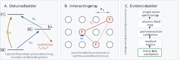
A Rydberg array is a calibrated stack. A detuned ladder produces the effective $|g\rangle\leftrightarrow|r\rangle$ coupling but also light shifts and intermediate-state scattering. Pair interactions in the array become a usable Hamiltonian only after single-atom, field, pair, and readout calibrations.

Phase and Doppler Geometry

For two absorbed photons, the two-photon coupling carries the spatial phase

$$\Omega_{\mathrm{eff}}(\mathbf r) \propto \exp\!\left( i\mathbf k_{\mathrm{eff}}\cdot\mathbf r \right),$$

where $\mathbf k_{\mathrm{eff}}$ is the signed sum of the participating wavevectors. Atomic motion therefore produces a two-photon Doppler detuning

$$\delta_D = \mathbf k_{\mathrm{eff}}\cdot\mathbf v.$$

For a ladder driven by absorption of both photons,

$$\mathbf k_{\mathrm{eff}} = \mathbf k_1+\mathbf k_2.$$

Counterpropagating beams with unequal wavelengths reduce $|\mathbf k_{\mathrm{eff}}|$ but do not make it vanish. Copropagating beams increase the Doppler sensitivity. The geometry must also be compared with the trap axes: a cold atom can have different velocity widths along different directions, and local addressing beams can imprint site-dependent phases.

For a one-dimensional Maxwell distribution,

$$\sigma_v = \sqrt{\frac{k_{\mathrm B}T}{m}}, \qquad \frac{\sigma_D}{2\pi} = \frac{ |\mathbf k_{\mathrm{eff}}|\sigma_v }{ 2\pi }.$$

Cooling helps in two distinct ways. It narrows the Doppler distribution and reduces position-dependent sampling of the laser intensity and pair interaction. Neither effect is captured by quoting temperature alone; the relevant quantities are the motional distribution, trap frequencies, beam geometry, and pulse duration.

Worked Excitation Audit

Consider a simplified $^{87}\mathrm{Rb}$ ladder with

$$\begin{aligned} \frac{\Omega_1}{2\pi}&=100\ \mathrm{MHz}, & \frac{\Omega_2}{2\pi}&=20\ \mathrm{MHz}, \\ \frac{\Delta}{2\pi}&=1.0\ \mathrm{GHz}, & \frac{\Gamma_p}{2\pi}&=6.0\ \mathrm{MHz}. \end{aligned}$$

The effective Rabi frequency is

$$\frac{\Omega_{\mathrm{eff}}}{2\pi} \simeq \frac{ (100\ \mathrm{MHz})(20\ \mathrm{MHz}) }{ 2(1000\ \mathrm{MHz}) } = 1.0\ \mathrm{MHz},$$

so an ideal resonant pi pulse lasts

$$t_\pi = \frac{\pi}{\Omega_{\mathrm{eff}}} = 0.50\ \mu\mathrm s.$$

The light-shift scales are

$$\frac{\Delta_g^{\mathrm{AC}}}{2\pi} \simeq 2.5\ \mathrm{MHz}, \qquad \frac{\Delta_r^{\mathrm{AC}}}{2\pi} \simeq 0.10\ \mathrm{MHz}.$$

Their differential value is therefore about $2.4\ \mathrm{MHz}$ in magnitude, larger than $\Omega_{\mathrm{eff}}/(2\pi)$. A laser pair placed at the bare two-photon resonance would be substantially off resonance.

For an atom initially in $|g\rangle$, the leading intermediate-state population scale is

$$P_p \sim \frac{|\Omega_1|^2}{4\Delta^2} = 2.5\times10^{-3}.$$

Using the population decay rate $\Gamma_p=2\pi\times6.0\ \mathrm{MHz}$ gives

$$\Gamma_{\mathrm{sc}} \sim 9.4\times10^4\ \mathrm{s}^{-1}.$$

Multiplying this constant upper-scale estimate by $t_\pi$ gives about $4.7\%$. The true probability during a shaped population-transfer pulse must be obtained from the time-dependent multilevel master equation. The audit nevertheless exposes three facts before any fit is attempted:

1. the useful two-photon coupling is fast on a microsecond scale;
2. differential light shifts require explicit calibration or compensation;
3. intermediate-state scattering is not automatically negligible at a gigahertz detuning.

Now take counterpropagating $780\ \mathrm{nm}$ and $480\ \mathrm{nm}$ beams. For $T=10\ \mu\mathrm K$,

$$\sigma_v \simeq 3.09\times10^{-2}\ \mathrm{m\,s^{-1}},$$

and

$$\frac{\sigma_D}{2\pi} \simeq 24.8\ \mathrm{kHz}.$$

The copropagating geometry gives approximately $104\ \mathrm{kHz}$. Both are below the nominal $1\ \mathrm{MHz}$ Rabi frequency, but the larger value can still contribute measurable dephasing and site-to-site detuning variation.

This calculation is deliberately only a scale audit. Real $^{87}\mathrm{Rb}$ requires the intermediate hyperfine manifold, actual Clebsch–Gordan coefficients, beam waists, laser spectra, polarization impurities, and branching to states outside the chosen basis.

Electric Fields and Stark Maps

An isolated parity eigenstate with no permanent laboratory-frame dipole has a leading quadratic Stark shift

$$\Delta E_r = -\frac{1}{2}\alpha_r(0)E^2.$$

Because the Rydberg polarizability can be enormous, a field too small to matter for a ground-state transition can shift the Rydberg resonance by many linewidths. Near-degenerate manifolds require diagonalizing the Stark Hamiltonian; their response can become linear over an experimentally relevant range. A single scalar polarizability is then inadequate.

Compensation by spectroscopy

Suppose an electrode voltage $V$ produces field

$$E(V) = E_{\mathrm{stray}}+\beta(V-V_0).$$

In the quadratic regime, the transition frequency follows

$$\nu(V) = \nu_{\min} -\frac{\alpha_{\mathrm{diff}}}{2h} \left[ E_{\mathrm{stray}}+\beta(V-V_0) \right]^2.$$

The vertex identifies the compensation voltage only along the electrode’s field direction. Three-dimensional compensation requires independent field directions or a model of the electrode response matrix. Cross-couplings, voltage offsets, and patch charges make this a matrix calibration, not three unrelated knob scans.

An experimental Stark map serves several purposes:

• identifies the intended Rydberg state and nearby avoided crossings;
• measures the residual electric field and electrode response;
• reveals whether a quadratic approximation is valid;
• locates interaction resonances and unwanted pair channels; and
• tracks slow drift from surface charging, adsorbates, or photoelectrons.

Compensation is not permanent. Ultraviolet or blue excitation light can alter surface charge, and moving optics or changing trap power can change the local environment. Field scans belong in the repeated calibration schedule.

Magnetic fields matter as well. They define the quantization axis and lift Zeeman degeneracies, but field gradients and calibration errors create site-dependent detunings. Electric and magnetic shifts should be separated by their symmetry under field reversal and by spectroscopy of multiple states.

Population Lifetime and Coherence

Radiative and blackbody processes

For ordinary low-angular-momentum Rydberg series at zero temperature, the radiative lifetime often scales approximately as $(n^*)^3$. At finite temperature, ambient blackbody photons drive transitions to nearby Rydberg states and can contribute photoionization. A useful rate ledger is

$$\frac{1}{T_1} = \Gamma_{\mathrm{rad}} +\Gamma_{\mathrm{BBR}} +\Gamma_{\mathrm{photo}} +\Gamma_{\mathrm{coll}} +\cdots.$$

The terms depend on state, temperature, electromagnetic environment, atomic density, and applied light. A tabulated free-space lifetime is therefore not automatically the in-apparatus lifetime.

Lifetime is not coherence time

The coherence between $|g\rangle$ and $|r\rangle$ can decay faster than the Rydberg population:

$$\frac{1}{T_2} = \frac{1}{2T_1} +\Gamma_\phi.$$

Here $\Gamma_\phi$ collects pure dephasing from laser phase noise, Doppler shifts, electric-field noise, magnetic shifts, intensity fluctuations, interaction inhomogeneity, and unresolved state mixing. The equality is a Markovian two-level model; nonstationary noise can produce nonexponential Ramsey contrast and requires a noise-spectrum or filter-function treatment.

Three measurements answer different questions:

Measurement	Main information	Important caveat
delayed population survival	$T_1$ and transfer to dark channels	detector may not distinguish decay products
Ramsey contrast	inhomogeneous and low-frequency dephasing	includes shot-to-shot detuning drift
spin echo or dynamical decoupling	refocusable noise versus irreversible loss	pulse errors can mimic decoherence

A platform report should state which definition of coherence is used and whether the quoted time is a fitted envelope, a $1/e$ point, or a bound.

Trapping During Rydberg Excitation

The optical potential of state $|a\rangle$ is set by its dynamic polarizability:

$$U_a(\mathbf r) \simeq -\frac{1}{4} \alpha_a(\omega_L) |\mathcal E(\mathbf r)|^2.$$

Ground and Rydberg states generally have very different polarizabilities at a tweezer wavelength. The consequences include

• a differential transition shift;
• different trapping or antitrapping forces;
• position-dependent detuning across the atomic wavepacket;
• motional excitation during state changes; and
• possible photoionization or coupling to nearby Rydberg levels.

Dynamic Polarizability owns the frequency-dependent response theory. At the platform level there are three common strategies.

Turn the trap off

The tweezer is extinguished during the Rydberg pulse and restored before imaging. This suppresses trap-induced differential shifts, but the atom evolves freely:

$$\mathbf r(t) = \mathbf r(0)+\mathbf v(0)t.$$

Long dark windows reduce recapture and change pair separations. Trap switching can also impart parametric excitation if the timing or extinction is imperfect.

Leave the trap on

Continuous confinement improves recapture and position stability, but requires calibrating the Rydberg-state potential, differential light shift, and any photoionization. A single transition frequency measured at one trap depth does not establish that the potential is benign.

Engineer state-insensitive trapping

At selected wavelengths, polarizations, or dressed operating points, the differential polarizability can be reduced. Such “magic” conditions are state-specific and can be spoiled by tensor structure, nearby resonances, polarization impurity, or intensity variation. They must be demonstrated by spectroscopy and motional measurements for the states actually used.

Motion changes both drive and interaction

In a thermal wavepacket, the Rabi frequency, detuning, and interaction are random variables:

$$\Omega_i=\Omega(\mathbf r_i), \qquad \Delta_i=\Delta(\mathbf r_i,\mathbf v_i), \qquad V_{ij}=V(\mathbf r_i-\mathbf r_j).$$

Replacing them by mean values can overpredict contrast because coherent averaging is nonlinear. A reliable model samples the measured position and velocity distributions or propagates the motional degrees of freedom explicitly.

Long-Range Interactions as a Platform Resource

The atomic origin of resonant dipole–dipole and off-resonant van der Waals interactions is developed in Rydberg Atoms Basics. At the platform level, the essential question is whether a chosen pair state can be represented by a scalar potential

$$V_{ij} \simeq \frac{C_6}{R_{ij}^6}$$

over the experiment’s range of separation, angle, fields, and detuning.

That approximation can fail because

• several Zeeman pair states are coupled;
• the interaction is anisotropic;
• a Förster defect becomes comparable to a dipole coupling;
• external fields mix pair channels;
• higher multipoles matter at short range;
• atomic motion samples a broad range of $R$; or
• the laser couples to more than one molecular eigenpotential.

The remedy is not to fit an arbitrary effective $C_6$ to every dataset. First calculate or spectroscopically map the relevant pair eigenstates, then state the interval over which a reduced model is valid.

Sensitivity to position

For a van der Waals interaction,

$$\frac{\delta V}{V} \simeq -6\frac{\delta R}{R}.$$

At $R=5.0\ \mu\mathrm m$, a relative-separation uncertainty of $\sigma_R=50\ \mathrm{nm}$ gives

$$\frac{\sigma_V}{|V|} \simeq 6\frac{0.050}{5.0} = 0.060.$$

A seemingly small one-percent position uncertainty therefore produces a six-percent interaction uncertainty. Angular noise can add another first-order contribution when the potential is anisotropic.

Effective Array Hamiltonian

After single-atom and pair calibration, a commonly used rotating-frame model is

$$\begin{aligned} H ={}& \frac{\hbar}{2} \sum_i \left[ \Omega_i e^{i\phi_i} |r_i\rangle\langle g_i| + \Omega_i^* e^{-i\phi_i} |g_i\rangle\langle r_i| \right] \\ &- \hbar\sum_i \Delta_i n_i + \sum_{i<j}V_{ij}n_i n_j, \end{aligned}$$

where

$$n_i = |r_i\rangle\langle r_i|.$$

This Hamiltonian is experimentally meaningful only with a parameter map:

• $\Omega_i$ includes beam intensity, polarization, and atomic position;
• $\phi_i$ includes optical phase and site geometry;
• $\Delta_i$ includes programmed detuning plus Stark, Zeeman, Doppler, and light shifts;
• $V_{ij}$ comes from a stated pair-state model or measurement; and
• omitted loss and dephasing channels have measured bounds.

If $\Omega_i=\Omega$, $\Delta_i=\Delta$, and the phases can be gauged away, the two internal states map to a spin-$1/2$ model. But “realizes an Ising model” does not mean every term beyond that ideal model is absent. It means the residual terms are calculated, measured, or bounded over the reported operating region.

The one-canonical-home rule matters here. Lattice Models Overview owns the many-body interpretation of lattice Hamiltonians. This page owns how the coefficients are prepared and validated in a Rydberg apparatus.

Excitation and Detection

Coherent excitation

A resonant Rabi trace is a necessary but incomplete diagnostic. For an ideal two-level atom initially in $|g\rangle$,

$$P_r(t) = \frac{\Omega^2}{\Omega^2+\Delta^2} \sin^2\!\left[ \frac{t}{2} \sqrt{\Omega^2+\Delta^2} \right].$$

Observed contrast loss can arise from decay, dephasing, detuning inhomogeneity, Rabi-frequency inhomogeneity, imperfect preparation, or readout. A damped sine fit may summarize the data but generally does not identify which mechanism dominates.

A useful single-atom characterization set contains

1. a frequency scan at several powers;
2. Rabi oscillations at several detunings;
3. Ramsey and echo measurements;
4. trap-depth and trap-off timing scans;
5. polarization and magnetic-field checks; and
6. independent readout calibration.

Loss-based detection

In many alkali tweezer experiments, ground-state atoms are recaptured and imaged, whereas Rydberg excitation tends to produce absence. Absence is not a projector onto $|r\rangle$. It can also result from ordinary background loss, heating, failed recapture, off-resonant transfer, ionization, or an imaging error.

Let $a$ denote the measured outcome “absent.” A binary confusion model is

$$\begin{pmatrix} P(a) \\ P(\bar a) \end{pmatrix} = \begin{pmatrix} P(a|g) & P(a|r) \\ P(\bar a|g) & P(\bar a|r) \end{pmatrix} \begin{pmatrix} P_g \\ P_r \end{pmatrix}.$$

The matrix must be calibrated under timing and trapping conditions close to those of the science sequence. Inverting it without propagating uncertainty can turn a small calibration error into a large population error.

More state-selective methods

Destructive field ionization directly detects charged fragments and can resolve arrival-time windows associated with different states. Rydberg de-excitation followed by recapture maps $|r\rangle$ back into a trapped state. Two-electron atoms can permit autoionization of the Rydberg electron, enabling state-selective detection while retaining additional internal information. Shelving and fluorescence protocols provide other mappings.

Every method has a transfer matrix. “High-fidelity detection” should specify which states are discriminated, whether the process is destructive, how leakage is treated, and how confidence intervals were obtained.

Worked Readout Correction

Suppose a ground-state atom survives and is detected with probability

$$s_g=0.98,$$

so $P(a|g)=0.02$. Suppose a prepared Rydberg atom is absent with probability

$$\ell_r=P(a|r)=0.95.$$

If the measured absent fraction is $P(a)=0.40$, then

$$P(a) = \ell_r P_r + (1-s_g)(1-P_r).$$

Solving,

$$P_r = \frac{ P(a)-(1-s_g) }{ \ell_r-(1-s_g) } = \frac{0.40-0.02}{0.95-0.02} \simeq 0.409.$$

Calling the raw absent fraction “$40\%$ Rydberg population” would be close in this example, but only accidentally. The correction grows when ordinary loss increases or Rydberg detection becomes less efficient. Correlated loss also invalidates a product of independent single-site confusion matrices.

Building a Rydberg Array

Preparation and rearrangement

A site-resolved array usually begins with stochastic loading. Imaging identifies occupied sites, movable tweezers rearrange atoms into a target geometry, and cooling reduces motional excitation. These operations are covered in Optical Tweezers. For Rydberg work, their output must be translated into distributions of position, velocity, internal state, and survival probability.

The target geometry is part of the Hamiltonian. Calibration must therefore include

• absolute site positions and magnification;
• relative-position fluctuations and drift;
• trap-depth uniformity;
• local Rabi-frequency and detuning maps;
• missing-site and rearrangement statistics; and
• correlations introduced by loading or transport.

Defect-free assembly does not imply defect-free dynamics. An atom can be present but internally misprepared, too hot, off resonance, or incorrectly classified at readout.

Pair calibration before many-body inference

A minimum pair program varies separation, orientation, electric field, and laser detuning. Observables can include double-excitation suppression, interaction-shifted resonances, coherent pair oscillations, or accumulated phase. Agreement at one separation is insufficient to establish an $R^{-6}$ law.

When the interaction is anisotropic, at least two noncollinear pair orientations are needed. When a Förster resonance is nearby, the electric field must be recorded and the multilevel pair spectrum retained. The pair measurement should use the same state preparation and readout corrections as the larger array.

Validation Ladder

The following order separates apparatus calibration from model inference.

1. Atomic identification

Resolve the intended transition, nearby magnetic sublevels, and relevant intermediate states. Compare measured frequencies and power dependences with an atomic-structure calculation.

2. Single-atom control

Measure spectra, Rabi dynamics, Ramsey contrast, population lifetime, and trap-dependent shifts. Fit jointly where possible so that one parameter set must explain several observables.

3. Field map

Acquire Stark spectra versus independent electrode voltages, identify the compensation point, and monitor it over time. Record magnetic-field and polarization settings.

4. Pair interaction

Measure pair response versus $R$, angle, and field. Compare a scalar $C_6/R^6$ fit with a multilevel pair-state calculation and state the accepted regime.

5. Readout matrix

Calibrate preparation and measurement errors using sequences that isolate ordinary loss, Rydberg loss, recapture, and dark-state transfer. Test whether errors are site-independent and uncorrelated.

6. Small-system closure

Predict two-, three-, or four-atom observables using parameters fixed above. Do not refit every many-body trace independently. Failure here often reveals a missing interaction channel or correlated noise.

7. Many-body validation

Use symmetry checks, conservation-law diagnostics, parameter reversals, subsystem comparisons, and classically tractable sizes. A quantum simulator does not validate itself merely by producing dynamics that are hard to calculate.

This ladder distinguishes three claims:

Claim	Required evidence
controllable Rydberg excitation	calibrated single-atom transfer and coherence
calibrated interacting array	single-atom evidence plus pair interactions, positions, and readout
faithful simulator or gate processor	array evidence plus task-specific validation and uncertainty

Error Budget

An honest error budget separates coherent model errors, stochastic noise, loss, and preparation-and-measurement effects.

Excitation errors

• laser-frequency and phase noise;
• pulse-area and pulse-shape errors;
• off-resonant intermediate and Rydberg levels;
• differential AC Stark shifts;
• spontaneous scattering from intermediate states;
• Doppler detuning and recoil; and
• imperfect polarization or quantization-axis alignment.

Rydberg-state errors

• radiative decay and blackbody-induced transitions;
• stray-field drift and electric-field noise;
• ionization or photoionization;
• collisions and molecular resonances; and
• state mixing near avoided crossings.

Trapping and motion errors

• trap-induced differential shifts;
• recapture failure during trap-off windows;
• thermal distributions of $\Omega_i$, $\Delta_i$, and $V_{ij}$;
• mechanical forces in state-dependent potentials;
• position drift and calibration uncertainty; and
• heating from switching or rearrangement.

Interaction-model errors

• finite blockade or unwanted double excitation;
• anisotropic and multilevel pair structure;
• uncertain $C_6$ or Förster defect;
• beyond-pairwise interactions;
• edge effects and missing atoms; and
• neglected long-range tails.

Preparation and measurement errors

• imperfect optical pumping;
• atom loss before the control sequence;
• false-positive and false-negative Rydberg outcomes;
• state leakage hidden by binary readout;
• correlated imaging or recapture errors; and
• postselection bias.

The entries should be converted into a common task metric only after their mechanisms are modeled. Adding all percentages linearly is conservative but can grossly overestimate independent errors; adding them in quadrature is unjustified for coherent biases. Process simulation, randomized protocols, or likelihood-based inference should preserve the distinction.

Common Mistakes

Treating high n as an unconditional improvement

Larger $n$ can strengthen interactions, but it also densifies the spectrum and increases electric-field sensitivity. The optimum is apparatus- and task-dependent.

Using n instead of effective principal quantum number

Alkali scaling laws are organized by $n^*=n-\delta_{\ell j}$. Comparing different angular series by printed $n$ alone can be misleading.

Dropping light shifts after eliminating the intermediate state

The same virtual coupling that creates $\Omega_{\mathrm{eff}}$ creates differential AC Stark shifts. The excitation audit above shows that the shift can exceed the effective Rabi frequency.

Mixing linewidth and decay-rate conventions

If $\Gamma/(2\pi)$ is quoted in megahertz, the population decay rate is $\Gamma$ in inverse seconds. Omitting $2\pi$ underestimates scattering probabilities by that factor.

Calling counterpropagating two-photon excitation Doppler-free

Unequal wavelengths leave a nonzero effective wavevector. Counterpropagation reduces, rather than generally eliminates, first-order Doppler sensitivity.

Treating a tabulated lifetime as the coherence time

$T_1$ limits $T_2$ but does not determine it. Laser phase noise, field noise, motion, and inhomogeneity can dominate coherence.

Treating atom absence as a Rydberg projector

Ordinary loss, failed recapture, and dark-state transfer also produce absence. A calibrated confusion matrix is required.

Using a scalar C6 everywhere

The $C_6/R^6$ form assumes a specified perturbative pair channel. Angular structure, Förster resonances, external fields, and short separations can invalidate it.

Inferring an array Hamiltonian from one Rabi trace

Single-atom oscillations do not calibrate pair interactions, spatial inhomogeneity, readout, or correlated noise. The validation ladder must be closed.

Reporting a many-body fit without parameter provenance

Parameters fitted independently to each many-body dataset can absorb missing physics. A stronger test predicts small- and many-body data from independently calibrated parameters.

Exercises

Exercise 1: Eliminate the intermediate state

Use the three-level Hamiltonian on this page. Assume real $\Delta$ and $|\Delta|\gg|\Omega_1|,|\Omega_2|,|\delta|$. Derive the leading effective Hamiltonian in the $(|g\rangle,|r\rangle)$ subspace. Identify the two-photon Rabi frequency and the two diagonal light shifts.

Solution

The amplitude equations are

$$\begin{aligned} i\dot c_g &= \frac{\Omega_1^*}{2}c_p, \\ i\dot c_p &= \frac{\Omega_1}{2}c_g -\Delta c_p +\frac{\Omega_2^*}{2}c_r, \\ i\dot c_r &= \frac{\Omega_2}{2}c_p -\delta c_r. \end{aligned}$$

At leading adiabatic order, set $\dot c_p\simeq0$:

$$c_p \simeq \frac{ \Omega_1 c_g+\Omega_2^*c_r }{ 2\Delta }.$$

Substitution gives

$$i\frac{d}{dt} \begin{pmatrix} c_g\\c_r \end{pmatrix} = \begin{pmatrix} \dfrac{|\Omega_1|^2}{4\Delta} & \dfrac{\Omega_1^*\Omega_2^*}{4\Delta} \\ \dfrac{\Omega_1\Omega_2}{4\Delta} & -\delta+\dfrac{|\Omega_2|^2}{4\Delta} \end{pmatrix} \begin{pmatrix} c_g\\c_r \end{pmatrix}.$$

Writing the off-diagonal element as $\Omega_{\mathrm{eff}}/2$ gives

$$\Omega_{\mathrm{eff}} = \frac{\Omega_1\Omega_2}{2\Delta},$$

with phases assigned according to the definitions of $\Omega_1$ and $\Omega_2$. The diagonal shifts are

$$\Delta_g^{\mathrm{AC}} = \frac{|\Omega_1|^2}{4\Delta}, \qquad \Delta_r^{\mathrm{AC}} = \frac{|\Omega_2|^2}{4\Delta}.$$

Changing the detuning convention changes their displayed signs but not the need to retain the differential shift.

Exercise 2: Audit a two-photon pi pulse

For

$$\frac{\Omega_1}{2\pi}=100\ \mathrm{MHz}, \quad \frac{\Omega_2}{2\pi}=20\ \mathrm{MHz}, \quad \frac{\Delta}{2\pi}=1.0\ \mathrm{GHz},$$

calculate $\Omega_{\mathrm{eff}}/(2\pi)$, $t_\pi$, and both AC Stark-shift scales. If $\Gamma_p/(2\pi)=6.0\ \mathrm{MHz}$, estimate the ground-like intermediate-state scattering probability by treating $P_p\simeq|\Omega_1|^2/(4\Delta^2)$ as constant during the pulse. Explain why this is only a scale estimate.

Solution

The effective Rabi frequency is

$$\frac{\Omega_{\mathrm{eff}}}{2\pi} = \frac{(100)(20)}{2(1000)}\ \mathrm{MHz} = 1.0\ \mathrm{MHz}.$$

Hence

$$t_\pi = \frac{1}{2(1.0\ \mathrm{MHz})} = 0.50\ \mu\mathrm s.$$

The shift magnitudes are

$$\frac{\Delta_g^{\mathrm{AC}}}{2\pi} = \frac{100^2}{4(1000)}\ \mathrm{MHz} = 2.5\ \mathrm{MHz},$$

and

$$\frac{\Delta_r^{\mathrm{AC}}}{2\pi} = \frac{20^2}{4(1000)}\ \mathrm{MHz} = 0.10\ \mathrm{MHz}.$$

The intermediate population scale is

$$P_p = \frac{100^2}{4(1000)^2} = 2.5\times10^{-3}.$$

The population decay rate is

$$\Gamma_p = 2\pi(6.0\times10^6)\ \mathrm{s}^{-1}.$$

Therefore

$$p_{\mathrm{sc}} \sim \Gamma_p P_p t_\pi \simeq 0.047.$$

The estimate freezes a state-dependent intermediate population, ignores the $|r\rangle$ contribution and interference, and neglects pulse shape, multilevel structure, and branching. A master-equation calculation is needed for a quantitative error probability.

Exercise 3: Compare Doppler geometries

For two-photon absorption using wavelengths $780\ \mathrm{nm}$ and $480\ \mathrm{nm}$, calculate $|\mathbf k_{\mathrm{eff}}|/(2\pi)$ for counterpropagating and copropagating beams. For $^{87}\mathrm{Rb}$ at $10\ \mu\mathrm K$, use $m=1.443\times10^{-25}\ \mathrm{kg}$ to calculate the one-dimensional rms Doppler width in hertz.

Solution

For counterpropagating beams,

$$\frac{k_{\mathrm{eff}}}{2\pi} = \left| \frac{1}{480\ \mathrm{nm}} -\frac{1}{780\ \mathrm{nm}} \right| \simeq 8.01\times10^5\ \mathrm{m}^{-1}.$$

For copropagating beams,

$$\frac{k_{\mathrm{eff}}}{2\pi} = \frac{1}{480\ \mathrm{nm}} +\frac{1}{780\ \mathrm{nm}} \simeq 3.37\times10^6\ \mathrm{m}^{-1}.$$

The one-axis thermal velocity is

$$\sigma_v = \sqrt{ \frac{ (1.380649\times10^{-23})(10^{-5}) }{ 1.443\times10^{-25} } } \simeq 3.09\times10^{-2}\ \mathrm{m\,s^{-1}}.$$

Thus

$$\frac{\sigma_D^{\mathrm{counter}}}{2\pi} \simeq (8.01\times10^5)(3.09\times10^{-2}) \simeq 24.8\ \mathrm{kHz},$$

whereas

$$\frac{\sigma_D^{\mathrm{co}}}{2\pi} \simeq (3.37\times10^6)(3.09\times10^{-2}) \simeq 104\ \mathrm{kHz}.$$

Counterpropagation reduces the width by a factor of about $4.2$, but the unequal wavelengths prevent complete cancellation.

Exercise 4: Locate a Stark-compensation point

A Rydberg transition has a quadratic shift

$$\Delta\nu(V) = -A(E_s+\beta V)^2,$$

with $A>0$. Show that the vertex occurs at $V_c=-E_s/\beta$. If spectra along one electrode direction find $V_c=0.36\ \mathrm V$ and $\beta=0.25\ \mathrm{V\,cm^{-1}\,V^{-1}}$, what component of stray electric field is compensated? Why does this not establish full three-dimensional compensation?

Solution

Differentiate:

$$\frac{d\Delta\nu}{dV} = -2A\beta(E_s+\beta V).$$

The derivative vanishes at

$$V_c = -\frac{E_s}{\beta}.$$

Therefore

$$E_s = -\beta V_c = -(0.25)(0.36)\ \mathrm{V\,cm^{-1}} = -0.090\ \mathrm{V\,cm^{-1}}.$$

The electrode compensates only the projection of the stray field along its response direction. Transverse components remain, and real electrodes can produce nonorthogonal fields. A multidimensional voltage scan or calibrated electrode-response matrix is required.

Exercise 5: Distinguish T1 from T2

A Rydberg state has independent characteristic times

$$T_{\mathrm{rad}}=150\ \mu\mathrm s, \qquad T_{\mathrm{BBR}}=300\ \mu\mathrm s, \qquad T_{\mathrm{photo}}=1000\ \mu\mathrm s.$$

Calculate $T_1$. If the pure-dephasing time is $T_\phi=80\ \mu\mathrm s$, calculate $T_2$ using $1/T_2=1/(2T_1)+1/T_\phi$.

Solution

Independent population-loss rates add:

$$\frac{1}{T_1} = \frac{1}{150} +\frac{1}{300} +\frac{1}{1000} \quad \mu\mathrm s^{-1}.$$

Therefore

$$T_1 \simeq 90.9\ \mu\mathrm s.$$

The coherence time is

$$T_2 = \left[ \frac{1}{2(90.9)} +\frac{1}{80} \right]^{-1} \mu\mathrm s \simeq 55.6\ \mu\mathrm s.$$

The result is shorter than both $2T_1$ and $T_\phi$ because both mechanisms degrade coherence.

Exercise 6: Convert position noise into interaction noise

Two atoms interact through $V=C_6/R^6$. Linearize the interaction around $R_0$ and find the fractional rms interaction noise for $R_0=5.0\ \mu\mathrm m$ and $\sigma_R=50\ \mathrm{nm}$. If $|V(R_0)|/h=20\ \mathrm{MHz}$, estimate the rms frequency variation.

Solution

Differentiating,

$$\frac{dV}{dR} = -\frac{6C_6}{R^7} = -\frac{6V}{R}.$$

For small fluctuations,

$$\frac{\sigma_V}{|V|} \simeq 6\frac{\sigma_R}{R_0} = 6\frac{0.050}{5.0} = 0.060.$$

The interaction-frequency variation is therefore

$$\frac{\sigma_V}{h} \simeq 0.060(20\ \mathrm{MHz}) = 1.2\ \mathrm{MHz}.$$

This linear estimate assumes a narrow, approximately Gaussian radial distribution and ignores angular dependence.

Exercise 7: Correct loss-based detection

The probability that a ground-state atom appears absent is $0.02$, and the probability that a Rydberg atom appears absent is $0.95$. An experiment measures an absent fraction of $0.40$.

1. Infer the Rydberg population.
2. Repeat for an absent fraction of $0.04$.
3. Explain why the second inference is especially sensitive to calibration uncertainty.

Solution

The readout equation is

$$p_a = 0.02(1-p_r)+0.95p_r = 0.02+0.93p_r.$$

For $p_a=0.40$,

$$p_r = \frac{0.40-0.02}{0.93} \simeq 0.409.$$

For $p_a=0.04$,

$$p_r = \frac{0.04-0.02}{0.93} \simeq 0.0215.$$

In the second case, the signal above the ground-state loss floor is only $0.02$. A small error in that floor is comparable to the inferred Rydberg population. Confidence intervals must therefore propagate calibration counts and any drift, rather than treating $0.02$ and $0.95$ as exact constants.

Exercise 8: Design an array-validation package

An experiment claims to realize the Hamiltonian

$$H = \frac{\hbar\Omega}{2} \sum_i \left( |r_i\rangle\langle g_i|+\mathrm{h.c.} \right) -\hbar\Delta\sum_i n_i + \sum_{i<j} \frac{C_6}{R_{ij}^6} n_i n_j.$$

Design a minimal validation package that would support this claim without fitting $\Omega$, $\Delta$, and $C_6$ independently to every many-body trace. Include at least one test for each Hamiltonian term and one test of the measurement model.

Solution

A defensible package could contain:

1. Drive term: single-atom Rabi oscillations and power scaling at several sites, providing $\Omega_i$ and its spatial distribution.
2. Detuning term: single-atom spectra versus programmed detuning, trap power, electric field, and magnetic field, providing the calibrated $\Delta_i$ map.
3. Interaction term: two-atom spectroscopy or coherent dynamics over several separations and at least two angles, testing both the magnitude and $R^{-6}$ dependence of $C_6$.
4. Geometry: independent imaging calibration and repeated position measurements, providing $R_{ij}$ and its uncertainty.
5. Readout: prepared ground-like and Rydberg-like sequences that determine false-absence and false-presence probabilities, including tests for correlated loss.
6. Small-system closure: predict two-, three-, and four-atom observables using only the independently calibrated parameters.
7. Many-body checks: compare tractable system sizes, reverse detuning or geometry where symmetry predicts a change, and propagate all calibration uncertainties to observable bands.

The crucial feature is parameter provenance. The many-body comparison tests the Hamiltonian because its parameters were fixed before the comparison, rather than absorbed into a separate fit for every trace.

References

1. T. F. Gallagher, Rydberg Atoms (Cambridge University Press, 1994), doi:10.1017/CBO9780511524530.
2. T. F. Gallagher, “Rydberg atoms,” Reports on Progress in Physics 51, 143–188 (1988), doi:10.1088/0034-4885/51/2/001.
3. M. Saffman, T. G. Walker, and K. Mølmer, “Quantum information with Rydberg atoms,” Reviews of Modern Physics 82, 2313–2363 (2010), doi:10.1103/RevModPhys.82.2313.
4. M. Saffman, “Quantum computing with atomic qubits and Rydberg interactions: progress and challenges,” Journal of Physics B 49, 202001 (2016), doi:10.1088/0953-4075/49/20/202001.
5. C. S. Adams, J. D. Pritchard, and J. P. Shaffer, “Rydberg atom quantum technologies,” Journal of Physics B 53, 012002 (2020), doi:10.1088/1361-6455/ab52ef.
6. A. Browaeys and T. Lahaye, “Many-body physics with individually controlled Rydberg atoms,” Nature Physics 16, 132–142 (2020), doi:10.1038/s41567-019-0733-z.
7. I. I. Beterov, I. I. Ryabtsev, D. B. Tretyakov, and V. M. Entin, “Quasiclassical calculations of blackbody-radiation-induced depopulation rates and effective lifetimes of Rydberg $nS$, $nP$, and $nD$ alkali-metal atoms with $n\leq80$,” Physical Review A 79, 052504 (2009); erratum 80, 059902 (2009), doi:10.1103/PhysRevA.79.052504.
8. D. Jaksch, J. I. Cirac, P. Zoller, S. L. Rolston, R. Côté, and M. D. Lukin, “Fast quantum gates for neutral atoms,” Physical Review Letters 85, 2208–2211 (2000), doi:10.1103/PhysRevLett.85.2208.
9. E. Urban et al., “Observation of Rydberg blockade between two atoms,” Nature Physics 5, 110–114 (2009), doi:10.1038/nphys1178.
10. A. Gaëtan et al., “Observation of collective excitation of two individual atoms in the Rydberg blockade regime,” Nature Physics 5, 115–118 (2009), doi:10.1038/nphys1183.
11. L. Béguin et al., “Direct measurement of the van der Waals interaction between two Rydberg atoms,” Physical Review Letters 110, 263201 (2013), doi:10.1103/PhysRevLett.110.263201.
12. S. Ravets et al., “Coherent dipole–dipole coupling between two single Rydberg atoms at an electrically-tuned Förster resonance,” Nature Physics 10, 914–917 (2014), doi:10.1038/nphys3119.
13. D. Barredo et al., “An atom-by-atom assembler of defect-free arbitrary two-dimensional atomic arrays,” Science 354, 1021–1023 (2016), doi:10.1126/science.aah3778.
14. M. Endres et al., “Atom-by-atom assembly of defect-free one-dimensional cold atom arrays,” Science 354, 1024–1027 (2016), doi:10.1126/science.aah3752.
15. H. Bernien et al., “Probing many-body dynamics on a 51-atom quantum simulator,” Nature 551, 579–584 (2017), doi:10.1038/nature24622.
16. H. Levine et al., “High-fidelity control and entanglement of Rydberg-atom qubits,” Physical Review Letters 121, 123603 (2018), doi:10.1103/PhysRevLett.121.123603.
17. I. S. Madjarov et al., “High-fidelity entanglement and detection of alkaline-earth Rydberg atoms,” Nature Physics 16, 857–861 (2020), doi:10.1038/s41567-020-0903-z.
18. M. Morgado and S. Whitlock, “Quantum simulation and computing with Rydberg-interacting qubits,” AVS Quantum Science 3, 023501 (2021), doi:10.1116/5.0036562.
19. S. Ebadi et al., “Quantum phases of matter on a 256-atom programmable quantum simulator,” Nature 595, 227–232 (2021), doi:10.1038/s41586-021-03582-4.
20. P. Scholl et al., “Quantum simulation of 2D antiferromagnets with hundreds of Rydberg atoms,” Nature 595, 233–238 (2021), doi:10.1038/s41586-021-03585-1.

Cross-Links

• Neutral-Atom and Rydberg Qubits assembles the calibrated AMO ingredients into digital, analog, zone-based, loss-aware, and error-corrected processor architectures.
• Rydberg Array Frontiers gives a dated assessment of array scale, analog simulation, logical processing, erasure conversion, and the evidence still needed for advantage claims.
• AMO Platforms and Quantum Control places Rydberg arrays within the wider preparation–control–measurement cycle.
• Rydberg Atoms Basics develops the high-$n$ atomic structure and pair-interaction scaling used here.
• Optical Tweezers develops loading, imaging, rearrangement, and motional control of neutral atoms.
• Rydberg Blockade develops interaction-shifted two-atom dynamics, superatoms, blockade gates, and constrained many-body limits.
• Stark Effect in Atoms gives the canonical perturbative and degenerate-manifold treatment of electric fields.
• Rabi Oscillations develops coherent two-level driving and detuned response.
• Adiabatic Elimination develops the controlled reduction used for detuned ladder excitation.
• Neutral Atoms treats open-system models and measurement channels for neutral-atom platforms.
• AMO Physics Roadmap connects atomic structure, light–matter interaction, trapping, and many-body applications.