Ultracold Atoms

An ultracold atomic gas is an ensemble whose center-of-mass motion, collisions, and many-body correlations are governed by energy scales far below ordinary atomic electronic and often hyperfine splittings. In common laboratory usage, temperatures range from the low-microkelvin regime down to nanokelvin scales. The numerical temperature alone is not the definition.

The useful questions are dimensionless:

1. Is the collision wavelength long compared with the interaction range?
2. Do matter waves overlap, so that Bose or Fermi statistics affect the distribution?
3. Is the gas weakly interacting, resonant, or in a crossover between those regimes?
4. Are one or more motional directions energetically frozen?
5. Do elastic collisions establish equilibrium before loss, heating, or control ramps change the state?

These tests distinguish several claims that are often blurred together:

Claim	Representative criterion	What it does not establish
threshold collision regime	$kR\ll1$	quantum degeneracy
dilute gas	$nR^3\ll1$	weak scattering if $\lvert a\rvert\gg R$
quantum-degenerate gas	$n\lambda_{\mathrm{dB}}^3\gtrsim1$ or $T/T_{\mathrm F}\lesssim1$	condensation or superfluidity
weakly interacting Bose gas	$n\lvert a\rvert^3\ll1$, away from instability	ideal-gas behavior at every scale
resonant Fermi gas	$k_{\mathrm F}\lvert a\rvert\gg1$ with small range corrections	absence of loss or finite-temperature effects
lower-dimensional gas	active energies $\ll\hbar\omega_\perp$	validity of unmodified three-dimensional interactions

No single row implies all the others. A cloud can be ultracold but nondegenerate, degenerate but normal, dilute but strongly interacting, or geometrically thin while occupying many transverse modes.

Canonical Scope

This page owns the experimental and conceptual bridge from prepared cold atoms to interacting quantum gases. It develops:

1. operational degeneracy scales for bosons and fermions;
2. the role of the scattering length in dilute gases;
3. the control logic and limitations of magnetic Feshbach resonances;
4. trap, local-density, and dimensional-freezing audits;
5. the second-quantized Hamiltonian that connects AMO controls to many-body models;
6. preparation, thermometry, measurement, and uncertainty checks.

Scattering Length and Low-Energy Scattering own the threshold scattering derivations. Multichannel Scattering Preview and Feshbach Projection Formalism own the channel-space and projection-operator structures behind a resonance.

Bose–Einstein Condensation, Degenerate Fermi Gas, and Quantum Gases in Traps own the corresponding statistical-mechanical derivations. Here those results serve as state-preparation and validation criteria.

The Energy Ledger

An ultracold-gas statement should identify the energies that remain active. Typical entries are

$$\begin{aligned} E_T &= k_{\mathrm B}T, & E_{\mathrm F} &= k_{\mathrm B}T_{\mathrm F}, \\ E_{\mathrm{trap},i} &= \hbar\omega_i, & E_{\mathrm{int}} &\sim gn \quad\text{or}\quad E_{\mathrm F}F(k_{\mathrm F}a), \\ E_{\mathrm{rec}} &= \frac{\hbar^2k_L^2}{2m}, & E_{\mathrm{drive}} &= \hbar\Omega . \end{aligned}$$

They must be compared with internal-state splittings, molecular binding energies, optical linewidths, and the van der Waals energy scale when those degrees of freedom participate.

Cooling usually freezes electronic excitation first. Hyperfine and Zeeman states may remain as controlled internal components, while translational motion becomes quantum mechanical. Calling the atoms “two-level systems” does not remove their motional Hilbert space, and calling the gas “ultracold” does not imply that every internal state is in its ground level.

Three length scales

For a nonrelativistic particle of mass $m$, use the thermal de Broglie wavelength convention

$$\lambda_{\mathrm{dB}} = \frac{h}{ \sqrt{2\pi m k_{\mathrm B}T} }.$$

The mean spacing in a uniform three-dimensional gas is of order

$$d = n^{-1/3}.$$

A short-range interaction has a microscopic range $R$, often represented by a van der Waals length for neutral ground-state atoms. The hierarchy

$$R \ll d \lesssim \lambda_{\mathrm{dB}}$$

describes a dilute, quantum-degenerate threshold gas. It is not automatic: $R\ll d$ says that simultaneous three-particle encounters are geometrically rare, while $\lambda_{\mathrm{dB}}\gtrsim d$ says that particle exchange and quantum statistics matter.

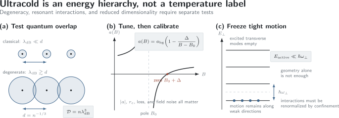
Three independent audits for an ultracold gas. Matter-wave overlap is measured by $\mathcal D=n\lambda_{\mathrm{dB}}^3$ or a Fermi degeneracy parameter. A Feshbach field tunes a low-energy parameter but also changes range, loss, and calibration requirements. Reduced dimensionality requires the occupied energy window to lie below $\hbar\omega_\perp$; a thin image alone is insufficient.

Degenerate Quantum Gases

The classical Maxwell–Boltzmann approximation fails when exchange cycles and occupation constraints affect observables. For a uniform one-component gas, the phase-space density is

$$\mathcal D = n\lambda_{\mathrm{dB}}^3.$$

The crossover begins around $\mathcal D\sim1$. For an ideal uniform three-dimensional Bose gas, excited states saturate at

$$\mathcal D_c = \zeta\!\left(\frac32\right) \simeq 2.612.$$

That number is not a universal experimental threshold. A harmonic trap has a different density of states, finite clouds round the transition, and interactions shift both density profiles and transition properties. The canonical trap formulas are on Quantum Gases in Traps.

Fermionic degeneracy scale

For one spin component of uniform density $n_\sigma$,

$$k_{\mathrm F,\sigma} = \left( 6\pi^2n_\sigma \right)^{1/3}, \qquad E_{\mathrm F,\sigma} = \frac{\hbar^2k_{\mathrm F,\sigma}^2}{2m}.$$

For a balanced two-component gas with total density $n=2n_\sigma$,

$$k_{\mathrm F} = \left( 3\pi^2n \right)^{1/3}, \qquad T_{\mathrm F} = \frac{E_{\mathrm F}}{k_{\mathrm B}}.$$

The degeneracy parameter is $T/T_{\mathrm F}$. A value much smaller than unity means that only excitations near the Fermi surface are thermally available. It does not by itself demonstrate pairing or superfluidity.

In a harmonic trap, one may instead quote a global shell-filling Fermi energy. That scale is not equal to the local $E_{\mathrm F}(\mathbf r)$ inferred from the density everywhere in the cloud. State which definition was used.

Bose and Fermi gases are not mirror images

Bosons can macroscopically occupy one orbital. Fermions fill distinct one-particle states and develop Fermi pressure even without interactions. For collisions:

• identical bosons may scatter in the $s$ wave;
• two distinguishable fermionic components may scatter in the $s$ wave;
• identical spin-polarized fermions cannot use an even spatial partial wave, so their low-energy $s$-wave collision channel is absent;
• higher partial waves are normally threshold-suppressed, although resonances can make them important.

This difference is central to cooling. Pauli blocking reduces available final states for collisions in a deeply degenerate Fermi gas, which can slow rethermalization. Fermions are therefore often evaporated in two-component mixtures or cooled sympathetically.

Worked scale comparison

Consider $^{87}\mathrm{Rb}$ at

$$T = 100\ \mathrm{nK}, \qquad n = 1.0\times10^{19}\ \mathrm{m}^{-3}.$$

Using $m=1.443\times10^{-25}\ \mathrm{kg}$ gives

$$\lambda_{\mathrm{dB}} \simeq 0.592\ \mu\mathrm m, \qquad d \simeq 0.464\ \mu\mathrm m,$$

and therefore

$$\mathcal D \simeq 2.08.$$

Quantum statistics are already important, but the ideal uniform Bose threshold has not quite been reached. Inferring condensation from this one number would still ignore trapping, interactions, finite size, and density calibration.

For a balanced two-state $^6\mathrm{Li}$ gas at the same total density,

$$k_{\mathrm F} \simeq 6.67\times10^6\ \mathrm{m}^{-1},$$

so

$$T_{\mathrm F} \simeq 1.79\ \mu\mathrm K.$$

At $T=200\ \mathrm{nK}$, the gas has $T/T_{\mathrm F}\simeq0.112$. The same numerical temperature can therefore represent very different degeneracy for different masses and densities.

Scattering Length as the Interaction Coordinate

At long wavelength, short-range two-body scattering is organized by the effective-range expansion

$$k\cot\delta_0(k) = - \frac1a + \frac12r_ek^2 + O(k^4).$$

The $s$-wave amplitude is

$$f_0(k) = \frac{1}{ -1/a+r_ek^2/2-ik }.$$

If $k|r_e|\ll1$, the leading approximation is

$$f_0(k) \simeq - \frac{a}{1+ika}.$$

This compression of microscopic chemistry into $a$ is one reason ultracold gases are controllable. It is a threshold expansion, not permission to discard every other length scale.

Cross sections and statistics

Neglecting effective-range corrections, distinguishable particles have

$$\sigma_{\mathrm{dist}}(k) = \frac{4\pi a^2}{ 1+k^2a^2 }.$$

For identical bosons in the same internal state, symmetrization gives

$$\sigma_{\mathrm B}(k) = \frac{8\pi a^2}{ 1+k^2a^2 },$$

under the standard total-cross-section convention. The factor of two is not an interaction enhancement; it follows from indistinguishable outgoing configurations.

When $k|a|\ll1$, the cross section is proportional to $a^2$. When $k|a|\gg1$, it no longer grows as $a^2$ but approaches the partial-wave unitarity scale proportional to $1/k^2$.

Contact coupling

For equal-mass particles in three dimensions, the dilute weak-coupling parameter commonly used for a Bose gas is

$$g = \frac{4\pi\hbar^2a}{m}.$$

The leading mean-field interaction energy is

$$\mu_{\mathrm{int}} \simeq gn.$$

The gas parameter

$$n|a|^3$$

measures diluteness relative to the scattering length. For a stable, weakly repulsive Bose gas, $na^3\ll1$ controls the expansion beyond mean field. A negative $a$ does not merely reverse a perturbative sign in a large homogeneous gas; attraction can cause mechanical instability, with finite traps supporting only limited metastable populations.

For a two-component Fermi gas, a standard interaction coordinate is

$$\frac{1}{ k_{\mathrm F}a }.$$

The regimes

$$\frac1{k_{\mathrm F}a} \ll -1, \qquad \frac1{k_{\mathrm F}a}=0, \qquad \frac1{k_{\mathrm F}a} \gg 1$$

label the BCS side, unitarity, and the molecular BEC side of the broad $s$-wave crossover, respectively. These labels assume a two-component gas, short effective range, and sufficient equilibrium. They do not apply unchanged to a single spin-polarized component.

What the sign of the scattering length says

The sign of $a$ describes the threshold phase shift, not the sign of the microscopic potential at every radius.

• Large positive $a$ commonly accompanies a shallow two-body bound state.
• Large negative $a$ commonly places the corresponding pole on the virtual side of threshold rather than as a physical shallow dimer.
• A potential containing both attraction and repulsion can have either sign of $a$.

For $a>0$ much larger than the interaction range, a universal shallow dimer has approximate binding energy

$$E_b \simeq \frac{\hbar^2}{ 2\mu_{\mathrm r}a^2 },$$

where $\mu_{\mathrm r}$ is the two-body reduced mass. For equal masses,

$$E_b \simeq \frac{\hbar^2}{ ma^2 }.$$

Effective-range, closed-channel, and finite-range corrections matter as $a$ becomes less dominant.

Limits of the one-parameter description

A scattering-length model needs revision when:

1. $k|r_e|$ is not small;
2. higher partial waves contribute;
3. several internal thresholds are nearby;
4. dipole–dipole, Coulomb, or other long-range forces remain active;
5. three-body parameters enter observables;
6. confinement changes the collision boundary conditions;
7. inelastic channels make $a$ complex or introduce separate loss coefficients.

“Universal” always means universal with respect to specified unresolved short-distance details, within a declared scale hierarchy.

Feshbach Resonances

A magnetic Feshbach resonance converts a magnetic field into an interaction control parameter. An incoming pair occupies an open channel. A different internal-state combination supports a closed-channel bound state whose energy shifts relative to the open-channel threshold because the two configurations have different magnetic moments. Coupling between channels causes resonant scattering when that dressed bound state approaches threshold.

Near an isolated resonance, a commonly used zero-energy parametrization is

$$a(B) = a_{\mathrm{bg}} \left( 1 - \frac{\Delta}{ B-B_0 } \right).$$

Here:

• $a_{\mathrm{bg}}$ is the background scattering length;
• $B_0$ is the pole position;
• $\Delta$ is the signed field width in this convention;
• the zero crossing occurs at $B=B_0+\Delta$.

Quoting $\Delta$ without the sign convention can reverse which side is called positive. Quoting the magnet power-supply setting without an independent field calibration does not establish $B-B_0$.

Pole, zero, and finite collision energy

The divergence in the zero-energy $a(B)$ formula is not a divergent physical cross section at finite momentum. At large $|a|$,

$$|f_0(k)|^2 \longrightarrow \frac1{k^2}$$

when range corrections are negligible. Temperature, density, confinement, and many-body effects therefore set the relevant momentum and cut off the zero-energy pole.

The zero crossing is useful for suppressing the leading contact interaction, but it does not eliminate:

• effective-range terms;
• residual interactions in other channels;
• dipolar interactions;
• three-body processes;
• state-dependent light shifts;
• technical heating.

Broad and narrow resonances

A resonance’s usefulness is not ranked by $\Delta$ in gauss alone. The physical comparison includes the differential magnetic moment, van der Waals scales, background scattering, and the resonance range parameter. Broad open-channel-dominated resonances can support a large interval where

$$k|r_e| \ll 1$$

and scattering-length universality is accurate. Narrow resonances retain stronger energy dependence and closed-channel character. Their effective range can become an essential many-body parameter.

Control is a trajectory

Changing $B$ can:

1. alter the elastic collision rate;
2. cross a molecular avoided crossing;
3. create or dissociate weakly bound dimers;
4. change three-body recombination;
5. release binding energy into untrapped products;
6. move the gas through a many-body crossover;
7. change equilibration and hydrodynamicity.

The ramp speed must therefore be compared with two-body association, many-body response, trap, collision, and loss timescales. “Adiabatic” is not a property of the waveform alone; it is relative to the gaps and relaxation processes relevant to the intended state.

A resonance audit

For a quantitative interaction claim, report at least:

Quantity	Why it matters
internal-state mixture	determines the open channel and allowed collisions
$B_0$, $\Delta$, $a_{\mathrm{bg}}$	defines the zero-energy calibration
field offset, noise, and gradients	map control electronics to interaction inhomogeneity
effective range or resonance-strength information	tests one-parameter universality
density and temperature	set typical collision momentum
two- and three-body loss	limit hold time and bias surviving samples
ramp history	determines association, heating, and nonequilibrium response

Loss maxima can help locate a resonance, but a loss feature is not by itself a precision measurement of the pole in the elastic scattering amplitude.

Traps, Inhomogeneity, and Dimensionality

Near a stable minimum, a smooth trap is often approximated by

$$V(\mathbf r) = \frac{m}{2} \left( \omega_x^2x^2 + \omega_y^2y^2 + \omega_z^2z^2 \right).$$

The oscillator lengths are

$$a_i = \sqrt{ \frac{\hbar}{ m\omega_i } }.$$

These lengths determine ground-state wave-packet sizes and compare confinement with scattering scales. They are distinct from thermal cloud radii and from interaction-broadened condensate radii.

A trap creates many local gases

In the local-density approximation,

$$\mu_{\mathrm{loc}}(\mathbf r) = \mu_0 - V(\mathbf r).$$

The center can be strongly degenerate while the wings remain classical. Likewise, a trapped interacting gas can sample several parts of a homogeneous phase diagram in one image. An average density inserted into a uniform-gas formula generally does not reproduce this structure.

LDA requires the potential to vary slowly on the local correlation length. It can fail near small clouds, sharp edges, critical regions, low-density boundaries, or microscopic lattice structure.

Geometry is not dimensionality

Suppose one direction has tight frequency $\omega_\perp$. Subtract the transverse zero-point energy and define an active many-body window

$$E_{\mathrm{active}} = \max \left\{ k_{\mathrm B}T,\, E_{\mathrm F}^{\parallel},\, |\mu_{\mathrm{int}}|,\, \hbar/t_{\mathrm{drive}} \right\}.$$

A controlled freeze-out criterion is

$$E_{\mathrm{active}} \ll \hbar\omega_\perp.$$

One frozen direction gives a quasi-two-dimensional gas. Two frozen directions give a quasi-one-dimensional gas. The symbol $E_{\mathrm F}^{\parallel}$ denotes the Fermi scale associated with the remaining weak directions; all chemical potentials here are measured relative to the transverse ground level.

A cigar-shaped or pancake-shaped density profile is not sufficient evidence. A hot anisotropic classical gas can have the same shape while occupying many tight-direction levels.

Confinement changes interactions

Even when transverse excitations are absent from the real population, virtual transverse excitation affects collisions. Effective one- and two-dimensional couplings depend on both

$$\frac{a}{ a_\perp } \quad\text{and}\quad \hbar\omega_\perp.$$

This produces confinement-induced renormalization and, in one dimension, a confinement-induced resonance. Substituting the three-dimensional $g=4\pi\hbar^2a/m$ directly into a one-dimensional Hamiltonian is generally incorrect.

Low-Dimensional Quantum Gases owns the state-counting, infrared, and interaction analysis. The operational lesson here is to calibrate both transverse occupation and the effective low-dimensional coupling.

Worked confinement check

For $^{87}\mathrm{Rb}$ with

$$\frac{\omega_\perp}{2\pi} = 50\ \mathrm{kHz},$$

the tight-direction level spacing is

$$\frac{\hbar\omega_\perp}{k_{\mathrm B}} = \frac{h(50\ \mathrm{kHz})}{k_{\mathrm B}} \simeq 2.40\ \mu\mathrm K.$$

The oscillator length is

$$a_\perp \simeq 48.2\ \mathrm{nm}.$$

A cloud with $T=100\ \mathrm{nK}$ and $\mu_{\mathrm{int}}/k_{\mathrm B}=300\ \mathrm{nK}$ is plausibly in the transverse ground mode, because both scales lie well below $2.40\ \mu\mathrm K$. That conclusion should still be checked spectroscopically or through a calibrated excited-mode fraction, especially after rapid loading or strong driving.

Harmonic, box, and lattice confinement

Different potentials answer different questions:

• Harmonic traps are smooth and experimentally common, but spatially inhomogeneous.
• Optical box traps approach uniform density over a central region and simplify equation-of-state comparisons, while walls and residual roughness remain finite.
• Optical lattices create bands, tunneling, and on-site interactions; they are not merely tight continuum traps.
• Tweezers emphasize programmable few-body or site-resolved preparation, with array uniformity and transport as additional controls.

The later optical-lattice platform page owns lattice implementation. Bose–Hubbard Model owns the canonical many-body model and its approximations.

Connection to Many-Body Quantum Mechanics

Once internal electronic excitations and microscopic collision structure are integrated out, a multicomponent continuum gas is often organized by

$$\begin{aligned} H ={}& \sum_\sigma \int d^dr\, \hat\psi_\sigma^\dagger(\mathbf r) \left[ - \frac{\hbar^2\nabla^2}{2m_\sigma} + V_\sigma(\mathbf r,t) \right] \hat\psi_\sigma(\mathbf r) \\ &+ \frac12 \sum_{\sigma,\sigma'} g_{\sigma\sigma'} \int d^dr\, \hat\psi_\sigma^\dagger \hat\psi_{\sigma'}^\dagger \hat\psi_{\sigma'} \hat\psi_\sigma + H_{\mathrm{long}} + H_{\mathrm{drive}} . \end{aligned}$$

All field operators in the interaction term are evaluated at $\mathbf r$. They obey commutation or anticommutation relations according to the isotope and chosen constituents.

The apparent delta interaction in three dimensions is an effective low-energy description. Its bare coupling requires regularization in ultraviolet-sensitive calculations. The experimentally meaningful scattering length fixes the renormalized low-energy amplitude.

Field Operators owns the operator construction. Gross–Pitaevskii Equation owns the weakly interacting condensate mean-field limit.

Experimental knobs become Hamiltonian terms

AMO control	Effective many-body coordinate
isotope and internal state	particle statistics, mass, component labels
magnetic field near a resonance	$a$, effective range, molecular detuning
atom number and trap shape	density, Fermi scale, inhomogeneity
transverse confinement	dimensionality and effective coupling
optical lattice depth	hopping, bandwidth, on-site interaction
state-dependent light shift	spin-dependent potential or field
Raman coupling	coherent intercomponent coupling, synthetic momentum transfer
controlled disorder	random or quasiperiodic potential
periodic modulation	Floquet drive and heating channels
imaging and loss	measurement backaction and open-system terms

This control is powerful but not unlimited. The realized Hamiltonian includes calibration errors, higher bands, residual confinement, photon scattering, loss, and finite entropy. A quantum simulator is validated by comparing those terms with the target-model scales, not by naming the target Hamiltonian.

Regime map

Ultracold atoms connect naturally to:

• Bose condensation and weakly interacting superfluids;
• the BCS–BEC crossover and unitary Fermi gas;
• one-dimensional Lieb–Liniger and Tonks–Girardeau regimes;
• Bose–Hubbard and Fermi–Hubbard physics in lattices;
• spin models derived in restricted filling and strong-coupling limits;
• nonequilibrium quenches, transport, hydrodynamics, and prethermalization;
• few-body universality and Efimov physics;
• dipolar and multicomponent quantum matter.

Each item requires additional assumptions. For example, a Hubbard model requires a justified band projection, while a spin model additionally requires controlled filling and an energy separation that suppresses charge fluctuations.

Preparation as a State-Engineering Chain

A common continuum-gas sequence is

$$\begin{gathered} \text{atomic source} \longrightarrow \text{laser slowing and MOT} \longrightarrow \text{sub-Doppler preparation} \\ \longrightarrow \text{conservative trap} \longrightarrow \text{evaporation or sympathetic cooling} \longrightarrow \text{interaction and geometry ramp} \longrightarrow \text{probe}. \end{gathered}$$

Evaporative Cooling owns selective loss, rethermalization, and phase-space-density efficiency. Optical Dipole Traps owns conservative trap depth, frequencies, scattering, gravity, and technical heating.

At each transfer, audit:

1. atom number and component populations;
2. temperature or entropy per particle;
3. density profile and trap frequencies;
4. phase-space density or $T/T_{\mathrm F}$;
5. elastic collision and rethermalization rate;
6. one-, two-, and three-body loss;
7. interaction calibration;
8. adiabaticity relative to relevant gaps;
9. spatial and internal-state purity.

A later state can contain fewer atoms and be colder yet have lower phase-space density. Likewise, an adiabatic trap decompression can lower $T$ without removing entropy per particle.

Observables and What They Infer

Ultracold-gas measurements usually infer a many-body quantity through a forward model.

Measurement	Common inference	Required qualification
absorption or phase-contrast image	column density	optical depth, saturation, detuning, point-spread function
time-of-flight image	momentum distribution	release dynamics, collisions, far-field condition
bimodal fit	condensate fraction	model choice, interactions, finite resolution
in situ equation of state	$T$, $\mu$, pressure, compressibility	LDA, potential calibration, imaging response
radio-frequency spectroscopy	pairing or excitation spectrum	final-state interactions, pulse response
Bragg spectroscopy	dynamic structure factor	momentum resolution and linear-response regime
noise correlations	occupation correlations	finite imaging transfer and ensemble averaging
site-resolved fluorescence	parity or occupation	light-assisted loss, reconstruction fidelity
collective modes	equation of state or hydrodynamics	excitation amplitude, damping model, anisotropy
atom loss	inelastic coefficient or resonance indicator	density calibration and competing channels

Thermometry is model dependent

At high enough temperature, a thermal wing can be fitted to a classical distribution. Near degeneracy, Bose or Fermi occupation factors must be used. Deep in a correlated regime, thermometry may rely on an equation of state, fluctuation relation, impurity, spin gradient, or adiabatic connection to a calibrated reference state.

The colder the gas, the less reliable a naive Gaussian width becomes. Report the thermometer, its calibration range, and whether it measures the state before or after an interaction or trap ramp.

Timescale closure

An equilibrium interpretation needs a window such as

$$\tau_{\mathrm{micro}} \ll \tau_{\mathrm{eq}} \ll \tau_{\mathrm{loss}}, \tau_{\mathrm{heat}}, \tau_{\mathrm{drift}}.$$

The microscopic time may be $\hbar/E_{\mathrm F}$, a trap period, a tunneling time, or an inverse collective-mode frequency. Equilibration can be much slower than a single collision, especially near integrability, with Pauli blocking, or after a large quench.

Holding longer without observing stationarity does not prove equilibrium. A useful test varies the hold time and preparation path while comparing several independent observables.

A Minimal Quantitative Report

A reproducible ultracold-gas state should specify:

$$\left\{ N_\sigma,\, T,\, \omega_i,\, n(\mathbf r),\, a,\, r_e,\, \tau_{\mathrm{loss}},\, \text{ramp history} \right\},$$

or the corresponding box- or lattice-potential parameters.

Derived dimensionless coordinates should include whichever are relevant:

$$\mathcal D, \qquad \frac{T}{T_{\mathrm F}}, \qquad n|a|^3, \qquad \frac1{k_{\mathrm F}a}, \qquad k_{\mathrm F}r_e, \qquad \frac{E_{\mathrm{active}}}{ \hbar\omega_\perp }.$$

Uncertainty propagation matters because these quantities combine measured inputs nonlinearly. For example,

$$\frac{\delta T_{\mathrm F}}{ T_{\mathrm F} } = \frac23 \frac{\delta n}{n}$$

to first order for a uniform gas if density is the only uncertain input. Near a Feshbach pole,

$$\frac{da}{dB} = a_{\mathrm{bg}} \frac{\Delta}{ (B-B_0)^2 },$$

so a fixed magnetic-field uncertainty can become a very large interaction uncertainty.

Common Mistakes

Defining ultracold by a temperature cutoff.
The relevant thresholds depend on mass, density, interaction range, and confinement.

Equating quantum degeneracy with condensation.
$\mathcal D\sim1$ marks the onset of exchange effects. Condensation has an additional criterion, and fermions do not condense as individual particles.

Using total density in a one-component Fermi formula without stating spin degeneracy.
Define whether $n$ is per component or summed over components.

Replacing the finite-energy cross section by $4\pi a^2$ near resonance.
The factor $1/(1+k^2a^2)$ and effective-range corrections prevent an unbounded physical cross section.

Calling the sign of $a$ the sign of the microscopic potential.
$a$ is a threshold parameter shaped by the full radial wavefunction.

Treating a loss peak as the elastic pole.
Loss depends on density, temperature, hold time, and inelastic pathways.

Classifying a resonance as broad from its width in gauss alone.
Broadness is dimensionless and compares resonance and van der Waals scales.

Calling a thin cloud two dimensional.
Transverse excited-state occupation and the hierarchy $E_{\mathrm{active}}/\hbar\omega_\perp$ must be checked.

Using a three-dimensional contact coupling after dimensional freeze-out.
Confinement renormalizes low-dimensional scattering.

Using an average trap density as a homogeneous equation of state.
The local chemical potential varies across the cloud.

Interpreting every expanded image as momentum space.
Interactions during expansion, finite flight time, and lensing pulses can change the mapping.

Calling a simulator exact.
Higher bands, residual confinement, dissipation, finite entropy, and measurement transfer functions require a quantitative error budget.

Decision Workflow

For a new ultracold-gas problem:

1. List the internal components, masses, and statistics.
2. Identify whether densities are local, central, averaged, or per component.
3. Compute $\lambda_{\mathrm{dB}}$, $\mathcal D$, or $T/T_{\mathrm F}$.
4. Compare typical $k$ with the interaction range and effective range.
5. Choose the interaction coordinate: $na^3$, $1/(k_{\mathrm F}a)$, a low-dimensional coupling, or a long-range parameter.
6. Calibrate the trap and test LDA or discrete-level assumptions.
7. Test dimensional freeze-out using energy ratios, not cloud shape.
8. Compare elastic, equilibration, drive, loss, and heating times.
9. Propagate the preparation through the measurement forward model.
10. State which many-body Hamiltonian is justified and which omitted terms bound its accuracy.

Canonical Connections

• Quantum Statistics Overview owns Bose and Fermi ensemble structure.
• Bose–Einstein Condensation owns the ideal-gas condensation criterion and its qualifications.
• Bose–Einstein Condensates Overview connects macroscopic occupation to effective-field models, coherence, collective modes, and laboratory evidence.
• Degenerate Fermi Gas owns Fermi pressure and low-temperature thermodynamics.
• Degenerate Fermi Gases Overview connects component-resolved Fermi scales to spin mixtures, Feshbach tuning, the BEC–BCS crossover, evidence levels, and quantum simulation.
• Quantum Gases in Traps owns trap state counting, LDA, and imaging formulas.
• Low-Dimensional Quantum Gases owns dimensional crossover, infrared fluctuations, and effective low-dimensional regimes.
• Scattering Length owns the threshold definition and pole interpretation.
• Multichannel Scattering Preview owns open and closed channels and the $S$-matrix perspective.
• Evaporative Cooling owns the route from a trapped thermal cloud toward degeneracy.

References

1. M. H. Anderson, J. R. Ensher, M. R. Matthews, C. E. Wieman, and E. A. Cornell, “Observation of Bose–Einstein condensation in a dilute atomic vapor,” Science 269, 198–201 (1995), doi:10.1126/science.269.5221.198.

2. K. B. Davis, M.-O. Mewes, M. R. Andrews, N. J. van Druten, D. S. Durfee, D. M. Kurn, and W. Ketterle, “Bose–Einstein condensation in a gas of sodium atoms,” Physical Review Letters 75, 3969–3973 (1995), doi:10.1103/PhysRevLett.75.3969.

3. B. DeMarco and D. S. Jin, “Onset of Fermi degeneracy in a trapped atomic gas,” Science 285, 1703–1706 (1999), doi:10.1126/science.285.5434.1703.

4. F. Dalfovo, S. Giorgini, L. P. Pitaevskii, and S. Stringari, “Theory of Bose–Einstein condensation in trapped gases,” Reviews of Modern Physics 71, 463–512 (1999), doi:10.1103/RevModPhys.71.463.

5. S. Giorgini, L. P. Pitaevskii, and S. Stringari, “Theory of ultracold atomic Fermi gases,” Reviews of Modern Physics 80, 1215–1274 (2008), doi:10.1103/RevModPhys.80.1215.

6. I. Bloch, J. Dalibard, and W. Zwerger, “Many-body physics with ultracold gases,” Reviews of Modern Physics 80, 885–964 (2008), doi:10.1103/RevModPhys.80.885.

7. C. Chin, R. Grimm, P. Julienne, and E. Tiesinga, “Feshbach resonances in ultracold gases,” Reviews of Modern Physics 82, 1225–1286 (2010), doi:10.1103/RevModPhys.82.1225.

8. W. Ketterle and N. J. van Druten, “Evaporative cooling of trapped atoms,” Advances in Atomic, Molecular, and Optical Physics 37, 181–236 (1996), doi:10.1016/S1049-250X(08)60101-9.

9. R. Grimm, M. Weidemüller, and Y. B. Ovchinnikov, “Optical dipole traps for neutral atoms,” Advances in Atomic, Molecular, and Optical Physics 42, 95–170 (2000), doi:10.1016/S1049-250X(08)60186-X.

10. M. Olshanii, “Atomic scattering in the presence of an external confinement and a gas of impenetrable bosons,” Physical Review Letters 81, 938–941 (1998), doi:10.1103/PhysRevLett.81.938.

11. M. A. Cazalilla, R. Citro, T. Giamarchi, E. Orignac, and M. Rigol, “One-dimensional bosons: From condensed matter systems to ultracold gases,” Reviews of Modern Physics 83, 1405–1466 (2011), doi:10.1103/RevModPhys.83.1405.

12. E. Braaten and H.-W. Hammer, “Universality in few-body systems with large scattering length,” Physics Reports 428, 259–390 (2006), doi:10.1016/j.physrep.2006.03.001.

13. M. J. H. Ku, A. T. Sommer, L. W. Cheuk, and M. W. Zwierlein, “Revealing the superfluid lambda transition in the universal thermodynamics of a unitary Fermi gas,” Science 335, 563–567 (2012), doi:10.1126/science.1214987.

14. W. S. Bakr, J. I. Gillen, A. Peng, S. Fölling, and M. Greiner, “A quantum gas microscope for detecting single atoms in a Hubbard-regime optical lattice,” Nature 462, 74–77 (2009), doi:10.1038/nature08482.

15. L. W. Cheuk, M. A. Nichols, M. Okan, T. Gersdorf, V. V. Ramasesh, W. S. Bakr, T. Lompe, and M. W. Zwierlein, “Quantum-gas microscope for fermionic atoms,” Physical Review Letters 114, 193001 (2015), doi:10.1103/PhysRevLett.114.193001.

16. C. J. Pethick and H. Smith, Bose–Einstein Condensation in Dilute Gases, 2nd ed., Cambridge University Press (2008), doi:10.1017/CBO9780511802850.

Exercises

1. Matter-wave overlap

A uniform one-component gas has

$$n = 5.0\times10^{18}\ \mathrm{m}^{-3}, \qquad \lambda_{\mathrm{dB}} = 0.70\ \mu\mathrm m.$$

Compute $\mathcal D$ and the mean spacing $d=n^{-1/3}$. Is the gas safely classical?

Solution

The phase-space density is

$$\begin{aligned} \mathcal D &= n\lambda_{\mathrm{dB}}^3 \\ &= \left( 5.0\times10^{18}\ \mathrm{m}^{-3} \right) \left( 0.70\times10^{-6}\ \mathrm m \right)^3 \\ &\simeq 1.72. \end{aligned}$$

The spacing is

$$d = n^{-1/3} \simeq 0.585\ \mu\mathrm m.$$

Thus $\lambda_{\mathrm{dB}}/d\simeq1.20$. The matter waves overlap and the gas is not safely in the Maxwell–Boltzmann regime. For bosons, the value is still below the ideal uniform condensation threshold $2.612$, but this comparison alone does not diagnose a trapped interacting sample.

2. Balanced Fermi-gas convention

Show that a balanced two-component Fermi gas with total density $n$ has

$$k_{\mathrm F} = \left( 3\pi^2n \right)^{1/3}.$$

Explain why using $(6\pi^2n)^{1/3}$ would be inconsistent if $n$ is the total density.

Solution

Each component has density

$$n_\sigma = \frac n2.$$

For one component,

$$k_{\mathrm F} = \left( 6\pi^2n_\sigma \right)^{1/3}.$$

Substituting $n_\sigma=n/2$ gives

$$k_{\mathrm F} = \left( 3\pi^2n \right)^{1/3}.$$

The expression $(6\pi^2n)^{1/3}$ would treat the total density as though every particle occupied one spin component. It would overestimate $k_{\mathrm F}$ by $2^{1/3}$ and $E_{\mathrm F}$ by $2^{2/3}$.

3. Finite-energy unitarity correction

For distinguishable particles with negligible effective range, compare the finite-energy cross section at $k|a|=1$ with the threshold approximation $4\pi a^2$.

Solution

The finite-energy expression is

$$\sigma(k) = \frac{4\pi a^2}{ 1+k^2a^2 }.$$

At $k|a|=1$,

$$\sigma(k) = \frac{4\pi a^2}{2} = 2\pi a^2.$$

It is one half of the threshold approximation. Thus $4\pi a^2$ is already a poor estimate when $k|a|$ reaches unity.

4. Pole, zero, and sign

An isolated resonance is described by

$$a(B) = a_{\mathrm{bg}} \left( 1 - \frac{\Delta}{ B-B_0 } \right),$$

with $a_{\mathrm{bg}}=100a_0$ and $\Delta=20\ \mathrm G$. Find the zero crossing and evaluate $a$ at $B=B_0+4\ \mathrm G$.

Solution

The zero satisfies

$$1 - \frac{\Delta}{ B-B_0 } = 0,$$

so

$$B_{\mathrm{zero}} = B_0+\Delta = B_0+20\ \mathrm G.$$

At $B=B_0+4\ \mathrm G$,

$$\begin{aligned} a &= 100a_0 \left( 1-\frac{20}{4} \right) \\ &= -400a_0. \end{aligned}$$

The negative result does not mean the microscopic potential is everywhere attractive. It states the sign of the threshold scattering parameter in that channel.

5. Universal dimer scaling

For two equal-mass atoms with large positive $a$, show how the shallow-dimer binding energy changes when $a$ is doubled. What assumption must be checked before trusting the result?

Solution

For equal masses,

$$E_b \simeq \frac{\hbar^2}{ ma^2 }.$$

Replacing $a$ by $2a$ gives

$$E_b(2a) = \frac14E_b(a).$$

The dimer becomes four times less deeply bound. This universal result assumes that $a$ is much larger than the interaction range and that effective-range and closed-channel corrections are small.

6. Dimensional freeze-out

A gas has

$$\frac{\omega_\perp}{2\pi} = 30\ \mathrm{kHz}, \qquad T = 150\ \mathrm{nK}, \qquad \frac{E_{\mathrm{int}}}{k_{\mathrm B}} = 400\ \mathrm{nK}.$$

Compare its largest quoted active energy with $\hbar\omega_\perp$. Is transverse freeze-out plausible?

Solution

The confinement spacing in temperature units is

$$\frac{\hbar\omega_\perp}{k_{\mathrm B}} = \frac{h(30\ \mathrm{kHz})}{k_{\mathrm B}} \simeq 1.44\ \mu\mathrm K.$$

The largest quoted active scale is

$$\frac{E_{\mathrm{active}}}{k_{\mathrm B}} \simeq 0.40\ \mu\mathrm K.$$

Therefore

$$\frac{E_{\mathrm{active}}}{ \hbar\omega_\perp } \simeq 0.28.$$

Freeze-out is plausible but not asymptotically deep. A quantitative claim should measure or bound transverse excited-state occupation and include any Fermi, drive, or quench energy omitted from the question.

7. Local-density boundary

In an isotropic harmonic trap,

$$V(r) = \frac12m\omega^2r^2.$$

Within LDA, a homogeneous phase exists for $\mu_{\mathrm{loc}}>\mu_c$. Find the radius of its boundary in terms of $\mu_0$, $\mu_c$, $m$, and $\omega$.

Solution

The boundary obeys

$$\mu_{\mathrm{loc}}(r_c) = \mu_0 - \frac12m\omega^2r_c^2 = \mu_c.$$

Solving gives

$$r_c = \sqrt{ \frac{ 2(\mu_0-\mu_c) }{ m\omega^2 } },$$

provided $\mu_0>\mu_c$. The trap can therefore display a central phase and surrounding phases at lower local chemical potential in one equilibrium cloud.

8. Audit a “unitary two-dimensional gas” claim

An experiment describes a pancake-shaped two-component Fermi cloud as “a two-dimensional unitary gas” because it is tuned to the loss maximum near a known three-dimensional Feshbach resonance. List at least four additional checks needed to support the claim.

Solution

A defensible audit includes at least:

1. Dimensional freeze-out: compare $k_{\mathrm B}T$, the in-plane Fermi energy, interaction energy, and drive bandwidth with $\hbar\omega_\perp$; measure or bound transverse excited-state occupation.
2. Interaction calibration: calibrate $B$, $B_0$, field noise, and gradients. A loss maximum is not automatically the elastic pole.
3. Confinement-renormalized scattering: use the quasi-two-dimensional scattering amplitude or binding energy, not the bare three-dimensional $a(B)$ alone.
4. Range and loss: bound effective-range corrections and compare equilibration time with two- and three-body loss.
5. Component balance: measure spin populations and verify that the intended $s$-wave channel is present.
6. Thermodynamic state: report $T/T_{\mathrm F}$, density calibration, and evidence for equilibrium.

The shape of the cloud and proximity to a loss feature establish neither two-dimensionality nor universality by themselves.

Frontier Context

Ultracold Atom Quantum Simulation assesses current Hubbard, topological, gauge-theory, synthetic-dimension, and nonequilibrium simulations while preserving the platform and collision physics developed here as their canonical foundation.