Degenerate Fermi Gas

A Fermi gas is deeply degenerate when its temperature is much smaller than its Fermi temperature:

$$\theta \equiv \frac{T}{T_{\mathrm F}} \ll 1.$$

The dimensionless temperature $\theta$ is the central control parameter. It compares the thermal energy $k_{\mathrm B}T$ with the Fermi energy:

$$k_{\mathrm B}T_{\mathrm F} = \epsilon_{\mathrm F}.$$

Deep degeneracy does not mean that every particle is motionless. Even at $T=0$, the Pauli exclusion principle forces fermions to occupy a filled region of momentum space with a nonzero kinetic energy and pressure. Nor does degenerate mean that the many-body ground state must have several states of exactly equal energy. In this context, quantum degeneracy means that wave packets overlap strongly and Fermi–Dirac statistics controls the macroscopic state.

The organizing fact is simple:

At $T\ll T_{\mathrm F}$, almost all one-particle states far below the Fermi energy remain filled, almost all states far above it remain empty, and only a thin energy shell of width $O(k_{\mathrm B}T)$ can change its occupation.

That thin shell explains why:

• the heat capacity and entropy are proportional to $T/T_{\mathrm F}$;
• scattering is restricted by occupied final states;
• density fluctuations are suppressed;
• the zero-temperature pressure remains large;
• low-energy response is concentrated near the Fermi surface.

This page owns the physical interpretation of the degenerate regime and its application to electrons in metals, ultracold atoms, and white dwarfs. The Ideal Fermi Gas page owns the complete three-dimensional free-gas state counting and equation of state. Fermi Momentum and Fermi Energy gives the dimension-by-dimension reference formulas, Fermi Surface develops the boundary geometry and local low-energy kinematics, and Sommerfeld Expansion derives the asymptotic method behind the low-temperature coefficients quoted here.

Reference Model and Conventions

Unless stated otherwise, use:

• a uniform three-dimensional gas;
• noninteracting spinless or internally degenerate fermions;
• nonrelativistic dispersion;
• volume $V$ and density $n=N/V$;
• internal degeneracy $g$;
• the thermodynamic limit;
• fixed $N$ and $V$ when differentiating the low-temperature energy.

The one-particle dispersion is

$$\epsilon_k = \frac{\hbar^2k^2}{2m}.$$

At $T=0$, all modes inside the Fermi sphere are occupied:

$$f_{\mathrm F}(\epsilon) = \Theta(\epsilon_{\mathrm F}-\epsilon).$$

For the uniform three-dimensional model,

$$n = \frac{gk_{\mathrm F}^3}{6\pi^2},$$ $$\epsilon_{\mathrm F} = \frac{\hbar^2k_{\mathrm F}^2}{2m},$$

and

$$v_{\mathrm F} = \frac{\hbar k_{\mathrm F}}{m}.$$

These formulas define the reference scales. The focused Fermi-momentum page will own their dimensional and convention variants.

Equivalent Degeneracy Diagnostics

Several diagnostics express the same scale separation for the ideal three-dimensional gas.

Small reduced temperature

The most direct statement is

$$\theta = \frac{T}{T_{\mathrm F}} \ll 1.$$

Large phase-space density

Define the thermal de Broglie wavelength

$$\lambda_T = \sqrt{ \frac{2\pi\hbar^2}{mk_{\mathrm B}T} }.$$

Using the zero-temperature density relation,

$$\frac{n\lambda_T^3}{g} = \frac{4}{3\sqrt\pi} \left( \frac{T_{\mathrm F}}{T} \right)^{3/2}.$$

Therefore

$$T \ll T_{\mathrm F}$$

implies

$$\frac{n\lambda_T^3}{g} \gg 1.$$

The opposite limit, $n\lambda_T^3/g\ll1$, is the Maxwell–Boltzmann regime developed on the Maxwell–Boltzmann Limit page.

Large fugacity

The fugacity is

$$z = e^{\beta\mu}.$$

At low temperature and fixed density,

$$\mu \approx \epsilon_{\mathrm F},$$

so

$$\beta\mu \sim \frac{T_{\mathrm F}}{T} \gg 1$$

and $z\gg1$. A low-temperature degenerate gas is therefore not described by an expansion in small fugacity.

The Chemical Potential page develops the fixed-density meaning of $\mu(T)$ and its zero-temperature addition-energy limit.

Sharp occupation edge

The Fermi–Dirac occupation is

$$f(\epsilon) = \frac{1}{ e^{\beta(\epsilon-\mu)}+1 }.$$

Its crossover from nearly one to nearly zero occurs in an energy window of order $k_{\mathrm B}T$ around $\mu$.

Diagnostic	Degenerate regime
reduced temperature	$T/T_{\mathrm F}\ll1$
phase-space density per component	$n\lambda_T^3/g\gg1$
fugacity	$z\gg1$
chemical potential	$\mu\simeq\epsilon_{\mathrm F}>0$
occupation profile	sharp Fermi edge

The numerical boundaries between “classical,” “crossover,” and “deeply degenerate” depend on the desired accuracy. The symbol $\ll$ should be tied to an error tolerance, not interpreted as one universal decimal cutoff.

The Thermally Active Shell

Differentiate the occupation:

$$-\frac{\partial f}{\partial\epsilon} = \frac{1}{4k_{\mathrm B}T} \operatorname{sech}^2 \left[ \frac{\epsilon-\mu}{2k_{\mathrm B}T} \right].$$

This function is sharply localized near $\epsilon=\mu$ and has unit integral:

$$\int_{-\infty}^{\infty} d\epsilon\, \left( -\frac{\partial f}{\partial\epsilon} \right) = 1.$$

As $T\to0$,

$$-\frac{\partial f}{\partial\epsilon} \longrightarrow \delta(\epsilon-\epsilon_{\mathrm F})$$

in the distributional sense. Low-temperature response integrals therefore sample the density of states and matrix elements at the Fermi energy.

Near $k_{\mathrm F}$,

$$\epsilon_k-\epsilon_{\mathrm F} \approx \hbar v_{\mathrm F} (k-k_{\mathrm F}).$$

An energy window

$$\delta\epsilon \sim k_{\mathrm B}T$$

corresponds to a momentum-shell thickness

$$\delta k \sim \frac{k_{\mathrm B}T}{\hbar v_{\mathrm F}}.$$

For a quadratic dispersion,

$$\frac{\delta k}{k_{\mathrm F}} \sim \frac{1}{2} \frac{T}{T_{\mathrm F}}.$$

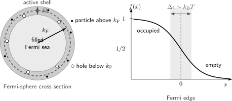
At $T\ll T_{\mathrm F}$, holes just inside $k_{\mathrm F}$ and particles just outside it occupy a shell with $\delta k/k_{\mathrm F}\sim T/(2T_{\mathrm F})$. The same shell appears in energy space as the rounded Fermi–Dirac edge of width $O(k_{\mathrm B}T)$ around $\mu$, with $x=(\epsilon-\mu)/(k_{\mathrm B}T)$.

The volume fraction of a thin spherical shell scales as

$$\frac{ 4\pi k_{\mathrm F}^2\delta k }{ (4\pi/3)k_{\mathrm F}^3 } \sim 3\frac{\delta k}{k_{\mathrm F}} \sim O\left( \frac{T}{T_{\mathrm F}} \right).$$

Only this order-$T/T_{\mathrm F}$ fraction of modes can participate freely in low-energy thermal rearrangements.

Particles and Holes

A fixed-$N$ thermal excitation removes a fermion from an occupied state below the Fermi surface and places it in an empty state above:

$$\text{filled state below} \longrightarrow \text{hole below} + \text{particle above}.$$

The hole is not a missing microscopic species. It is a useful description of the changed occupation relative to the filled reference sea. A particle and a hole near the Fermi surface can carry small excitation energy even though their individual momenta are of order $\hbar k_{\mathrm F}$.

Particle–Hole Excitations develops the operator state, signs of hole momentum and charge, continuum boundaries, and the way density and spin probes sum over these promotions.

This distinction is essential:

• the momentum of a thermally active fermion need not be small;
• the distance from the Fermi surface is small;
• low excitation energy means $|\epsilon-\mu|\lesssim k_{\mathrm B}T$, not $k\approx0$.

Pauli Blocking of Final States

Pauli exclusion constrains occupation numbers:

$$n_i \in \{0,1\}.$$

In a transition rate, this becomes a final-state availability factor. A one-particle transition from $i$ to $f$ carries the schematic statistical weight

$$f_i (1-f_f).$$

If the final mode is already occupied, $f_f=1$ and the process is blocked.

For two-body scattering,

$$1+2 \longrightarrow 3+4,$$

the occupation factor is

$$f_1f_2 (1-f_3) (1-f_4).$$

Energy and momentum conservation must be imposed in addition. At low temperature, most candidate final states below the Fermi surface are occupied, so the available scattering phase space collapses toward the thin thermal shell.

What blocking does not mean

Pauli blocking is not a repulsive force. It does not add a new potential to the Hamiltonian. It is a restriction on antisymmetric many-body states and on the availability of final modes.

It also does not mean that all collisions vanish:

• excited particles can scatter into available modes;
• different internal components can interact in the $s$ wave;
• impurities need not share the same blocked sea;
• collective processes can redistribute several excitations;
• finite temperature creates holes below the Fermi surface.

For a conventional Fermi liquid, the phase space for quasiparticle collisions near the Fermi surface often gives a low-temperature rate proportional to $T^2$. That statement requires interactions and quasiparticles; the exactly ideal gas has no collisions with which to equilibrate.

Two distinct antisymmetry effects

Do not conflate:

1. partial-wave restriction: identical spin-polarized fermions have no $s$-wave collision channel at ultralow energy;
2. many-body final-state blocking: occupied modes suppress otherwise allowed transitions in a filled Fermi sea.

The first is a two-body exchange-symmetry statement. The second depends on the many-body occupation distribution.

Suppressed Occupation Fluctuations

For one ideal fermionic mode,

$$\operatorname{Var}(n_i) = f_i(1-f_i).$$

Deep in the Fermi sea, $f_i\approx1$ and the variance is small. Far above it, $f_i\approx0$ and the variance is also small. Fluctuations are concentrated near $f_i=1/2$, inside the thermal shell.

Summing over modes gives

$$\operatorname{Var}(N) = \sum_i f_i(1-f_i)$$

in the grand-canonical ideal gas. Since

$$f(1-f) = k_{\mathrm B}T \left( -\frac{\partial f}{\partial\epsilon} \right),$$

the low-temperature scaling is

$$\operatorname{Var}(N) \sim k_{\mathrm B}T D(\epsilon_{\mathrm F}),$$

where $D(\epsilon_{\mathrm F})$ is the total density of states at the Fermi energy. Relative fluctuations are suppressed by $T/T_{\mathrm F}$.

The exact relation between number fluctuations and compressibility depends on the ensemble and volume under discussion. The general susceptibility framework belongs to Fluctuations and Susceptibilities.

Degeneracy Pressure

At $T=0$, a nonrelativistic ideal Fermi gas has

$$\frac{U_0}{N} = \frac{3}{5} \epsilon_{\mathrm F},$$

and

$$P_0 = \frac{2}{5} n\epsilon_{\mathrm F}.$$

This degeneracy pressure survives at zero temperature. It is not thermal pressure and not the result of pairwise repulsion.

Momentum-flux interpretation

For an isotropic gas with momentum $\mathbf p$, energy $\epsilon(p)$, and speed

$$v(p) = \frac{d\epsilon}{dp},$$

the pressure can be written

$$P = \frac{g}{3} \int \frac{d^3p}{(2\pi\hbar)^3} \, p\,v(p) f(p).$$

For

$$\epsilon(p) = \frac{p^2}{2m},$$

one has

$$p\,v(p) = \frac{p^2}{m} = 2\epsilon(p),$$

so

$$P = \frac{2U}{3V}.$$

The filled sea carries momentum flux even at $T=0$.

Density-scaling interpretation

Because

$$k_{\mathrm F} \propto n^{1/3},$$

the Fermi energy scales as

$$\epsilon_{\mathrm F} \propto n^{2/3}.$$

Therefore

$$\frac{U_0}{V} \propto n^{5/3}$$

and

$$P_0 \propto n^{5/3}.$$

Compression raises the momentum required to fit every fermion into a distinct state.

Uncertainty-scale interpretation

The mean spacing is $n^{-1/3}$. Localizing one fermion per available quantum cell suggests a momentum scale

$$p_{\mathrm F} \sim \hbar n^{1/3}.$$

Then

$$\frac{E}{N} \sim \frac{\hbar^2n^{2/3}}{m},$$

which again gives $P\sim n^{5/3}$. This argument captures the scaling but not the exact coefficient or degeneracy factor.

Compressibility at Zero Temperature

Since

$$P_0 \propto n^{5/3},$$

one finds

$$\frac{\partial P_0}{\partial n} = \frac{2}{3} \epsilon_{\mathrm F}.$$

The zero-temperature isothermal compressibility is

$$\kappa_T = \frac{1}{n} \left( \frac{\partial n}{\partial P} \right)_T = \frac{3}{2n\epsilon_{\mathrm F}}.$$

The gas is compressible, but not infinitely soft. Interactions and band structure alter this value in real systems.

Why the Heat Capacity Is Small

A classical monatomic gas has an order-$Nk_{\mathrm B}$ heat capacity because essentially every particle can explore thermally different energies. In a degenerate Fermi gas, particles deep in the sea cannot change state under a low-energy perturbation because nearby final modes are occupied.

The number of thermally active modes scales as

$$N_{\mathrm{active}} \sim D(\epsilon_{\mathrm F}) k_{\mathrm B}T.$$

Each active particle–hole excitation carries energy of order $k_{\mathrm B}T$. Therefore

$$U(T)-U(0) \sim D(\epsilon_{\mathrm F}) (k_{\mathrm B}T)^2,$$

and

$$C_V \sim D(\epsilon_{\mathrm F}) k_{\mathrm B}^2T.$$

The full Sommerfeld calculation fixes the coefficient. The underlying state-counting measure is developed on Density of States: First Encounter:

$$C_V = \frac{\pi^2}{3} D(\epsilon_{\mathrm F}) k_{\mathrm B}^2T + O(T^3).$$

For the uniform three-dimensional quadratic gas,

$$D(\epsilon_{\mathrm F}) = \frac{3N}{2\epsilon_{\mathrm F}},$$

so

$$C_V = \frac{\pi^2}{2} Nk_{\mathrm B} \frac{T}{T_{\mathrm F}} + O\left[ \left( \frac{T}{T_{\mathrm F}} \right)^3 \right].$$

The low-temperature entropy has the same leading coefficient:

$$S = \frac{\pi^2}{2} Nk_{\mathrm B} \frac{T}{T_{\mathrm F}} + O\left[ \left( \frac{T}{T_{\mathrm F}} \right)^3 \right].$$

Both vanish as $T\to0$, consistent with the third law for a nondegenerate ground state.

Leading Low-Temperature Corrections

For the three-dimensional nonrelativistic ideal gas at fixed density, let

$$\theta = \frac{T}{T_{\mathrm F}}.$$

The leading results are

$$\frac{\mu(T)}{\epsilon_{\mathrm F}} = 1 - \frac{\pi^2}{12} \theta^2 + O(\theta^4),$$ $$\frac{U(T)}{N} = \frac{3}{5} \epsilon_{\mathrm F} \left[ 1 + \frac{5\pi^2}{12} \theta^2 + O(\theta^4) \right],$$

and

$$P(T) = P_0 \left[ 1 + \frac{5\pi^2}{12} \theta^2 + O(\theta^4) \right].$$

The energy and pressure corrections begin at order $\theta^2$, while $C_V$ and $S$ begin at order $\theta$. Differentiation lowers the power by one.

These coefficients are not universal for every fermionic system. They depend on the dispersion, density of states, dimension, fixed variables, and interaction corrections. Sommerfeld Expansion owns the asymptotic derivation and its regularity assumptions.

Application: Electrons in Metals

For a representative monovalent free-electron density

$$n \approx 8.5\times10^{28}\ \mathrm{m}^{-3},$$

the spin-$1/2$ free-gas estimate gives

$$k_{\mathrm F} \approx 1.36\times10^{10}\ \mathrm{m}^{-1},$$ $$\epsilon_{\mathrm F} \approx 7.0\ \mathrm{eV},$$

and

$$T_{\mathrm F} \approx 8.2\times10^4\ \mathrm K.$$

At room temperature,

$$\frac{T}{T_{\mathrm F}} \approx 3.7\times10^{-3}.$$

The conduction electrons are therefore deeply degenerate even though the metal is nowhere near absolute zero.

Physical consequences

• Only electrons near the Fermi surface contribute efficiently to low-energy transport and thermal response.
• The electronic heat capacity is linear at low temperature:

$$C_{\mathrm{el}} = \gamma_{\mathrm{el}}T.$$

• Pauli blocking restricts electron–electron scattering phase space.
• The electron pressure and compressibility are set primarily by Fermi scales rather than by $k_{\mathrm B}T$.

The free-electron estimate is a benchmark, not a complete material model. In a crystal,

• the dispersion is a band energy $\epsilon_n(\mathbf k)$;
• the Fermi surface need not be spherical;
• effective masses can be anisotropic;
• several bands may cross the chemical potential;
• electron–electron and electron–phonon interactions renormalize observables.

Material-specific bands, transport, and ordered phases belong to Quantum Matter. This page retains only the generic degenerate-gas logic.

Application: Ultracold Fermionic Atoms

Cold-atom experiments can tune particle number, internal composition, trap geometry, and interactions. The natural thermometer is often the reduced temperature

$$\frac{T}{T_{\mathrm F}},$$

because an absolute temperature in nanokelvin says little without the density or trap scale.

For a homogeneous spin-polarized potassium-40 gas with illustrative density

$$n = 10^{18}\ \mathrm{m}^{-3},$$

the ideal-gas scales are approximately

$$k_{\mathrm F} \approx 3.9\times10^6\ \mathrm{m}^{-1},$$

and

$$T_{\mathrm F} \approx 92\ \mathrm{nK}.$$

A temperature of $20\ \mathrm{nK}$ would correspond to

$$\frac{T}{T_{\mathrm F}} \approx 0.22.$$

Observable signatures

• The momentum distribution approaches one particle per mode inside the Fermi surface for a single component.
• The cloud remains larger than a classical gas would at the same very low temperature because of Fermi pressure.
• Density fluctuations are suppressed by $f(1-f)$.
• Elastic scattering and evaporative cooling can slow as final states become blocked.
• Changing the number of spin components changes both collision channels and the density assigned to each Fermi sea.

In a harmonic trap, density and local Fermi energy vary with position. Quantum Gases in Traps owns the global trap Fermi scale, local-density profiles, and harmonic-level conventions.

Interaction scale

Degeneracy and interaction strength are independent questions. For a short-range two-component gas, a common interaction parameter is

$$k_{\mathrm F}a_s.$$

One can have:

• a weakly interacting degenerate gas;
• a strongly interacting degenerate gas;
• a paired superfluid with a gap;
• a classical but interacting gas.

The condition $T/T_{\mathrm F}\ll1$ alone does not make the ideal-gas approximation accurate.

Application: White Dwarfs

A white dwarf contains ions carrying most of the mass and electrons supplying much of the pressure support. Charge neutrality gives approximately

$$n_e = \frac{\rho}{\mu_e m_u},$$

where $\rho$ is the mass density, $m_u$ is the atomic mass unit, and $\mu_e$ is the mean mass per electron in units of $m_u$.

The star can be hot in everyday units while still satisfying

$$k_{\mathrm B}T \ll \epsilon_{\mathrm F,e}.$$

Its electrons are then deeply degenerate.

Nonrelativistic pressure

For spin-$1/2$ electrons,

$$k_{\mathrm F} = (3\pi^2n_e)^{1/3}.$$

In the nonrelativistic regime,

$$P_{\mathrm{NR}} = \frac{\hbar^2}{5m_e} (3\pi^2)^{2/3} n_e^{5/3}.$$

The exponent $5/3$ gives the familiar polytropic scaling. A rough hydrostatic estimate uses

$$P_{\mathrm{grav}} \sim \frac{GM^2}{R^4}$$

and

$$n_e \sim \frac{M}{ \mu_e m_u R^3 }.$$

Balancing $P_{\mathrm{NR}}$ against gravity gives

$$R \propto M^{-1/3}$$

at fixed composition, up to structure constants. More massive nonrelativistic white dwarfs are smaller.

Relativistic crossover

The nonrelativistic condition is

$$p_{\mathrm F} \ll m_ec.$$

As density grows, $p_{\mathrm F}$ becomes relativistic. For an ultrarelativistic ideal electron gas,

$$\epsilon(p) \approx pc,$$

and

$$P_{\mathrm{UR}} = \frac{\hbar c}{4} (3\pi^2)^{1/3} n_e^{4/3}.$$

The exponent changes from $5/3$ to $4/3$. Both ultrarelativistic degeneracy pressure and the characteristic gravitational pressure then scale as $R^{-4}$, so the radius drops out of the leading balance. The resulting mass scale is

$$M_{\mathrm{Ch}} \sim \frac{ (\hbar c/G)^{3/2} }{ (\mu_e m_u)^2 },$$

times a dimensionless structure coefficient.

This scaling argument explains why a limiting mass appears, but it is not a precision white-dwarf calculation. Composition, Coulomb corrections, inverse beta processes, finite temperature, rotation, magnetic fields, stellar structure, and general relativity refine the result. The standard idealized value is approximately

$$M_{\mathrm{Ch}} \approx \frac{5.83}{\mu_e^2} M_\odot,$$

which is about $1.46M_\odot$ for $\mu_e=2$.

Degenerate Does Not Mean Ideal

Real degenerate fermions often interact. The ideal Fermi gas remains useful because it supplies $k_{\mathrm F}$, $\epsilon_{\mathrm F}$, and the phase-space geometry against which interactions are measured.

Fermi-liquid regime

In a conventional Fermi liquid:

• low-energy excitations are quasiparticles near a Fermi surface;
• the heat capacity remains linear in $T$;
• an effective mass replaces the bare mass in some coefficients;
• compressibility and spin response contain interaction parameters;
• quasiparticle lifetimes grow as the surface is approached.

The scaling survives, but coefficients are renormalized.

Pairing

An attractive interaction can produce Cooper pairing and a superfluid or superconducting gap. Then the low-temperature heat capacity is no longer the gapless ideal-gas result. Degeneracy is a prerequisite for much pairing physics, not a guarantee that the normal ideal state remains stable.

Strong correlations

Near unitarity, in narrow bands, or near correlation-driven transitions, the ideal quasiparticle picture can fail quantitatively or qualitatively. A small $T/T_{\mathrm F}$ does not by itself control the interaction expansion.

Equilibrium and Timescales

The Fermi–Dirac distribution describes equilibrium. An exactly noninteracting gas cannot redistribute occupations and establish thermal equilibrium from an arbitrary initial state. In practice, weak interactions, collisions with another component, external noise, or preparation dynamics provide equilibration.

Deep degeneracy creates a tension:

• interactions are needed for thermalization;
• Pauli blocking suppresses the available final states;
• equilibration can therefore become slow as $T/T_{\mathrm F}$ decreases.

The equilibrium distribution and the relaxation time are different questions.

Validity Map

Question	Ideal degenerate-gas answer	Boundary
Is the gas quantum degenerate?	$T/T_{\mathrm F}\ll1$	crossover when the ratio is not small
Is the dispersion nonrelativistic?	$p_{\mathrm F}\ll mc$	relativistic equation of state
Is the gas uniform?	one global $k_{\mathrm F}$	traps and spatially varying density
Are interactions negligible?	separate coupling parameter is small	Fermi liquid, pairing, or strong correlation
Is a quadratic continuum dispersion valid?	free space or effective parabolic band	lattice bands and anisotropic Fermi surfaces
Is the Sommerfeld expansion controlled?	smooth density of states near $\mu$	band edges, singularities, gaps
Is equilibrium established?	relaxation is faster than observation	collisionless or prethermal state

Practical Workflow

For a degenerate-fermion estimate:

1. Specify dimension, dispersion, density per component, and internal degeneracy.
2. Compute $k_{\mathrm F}$ and $\epsilon_{\mathrm F}$ with one consistent convention.
3. Form $T/T_{\mathrm F}$.
4. Check the relativistic ratio $p_{\mathrm F}/(mc)$.
5. Estimate the active energy window $k_{\mathrm B}T$ and shell thickness.
6. Include final-state factors in transition and collision rates.
7. Use the zero-temperature pressure as the leading term and thermal corrections as powers of $T/T_{\mathrm F}$.
8. Check whether bands, traps, interactions, pairing, or finite size invalidate the uniform ideal model.
9. State whether the observable is evaluated at fixed $N$, fixed $\mu$, fixed volume, or fixed pressure.

Common Mistakes

Interpreting degeneracy as zero momentum

The Fermi sea contains momenta up to $p_{\mathrm F}$ at zero temperature.

Treating all particles as thermally active

Only an order-$T/T_{\mathrm F}$ shell can be rearranged by low-energy thermal processes.

Calling degeneracy pressure a repulsive interaction

The ideal gas has no pair potential. Its pressure follows from state filling and momentum flux.

Saying Pauli blocking stops every collision

Blocking depends on the actual final states, internal components, energy, and momentum conservation.

Confusing blocked final states with absent s-wave scattering

These are related to antisymmetry but are physically distinct restrictions.

Using the classical heat capacity

At low temperature,

$$C_V \propto N k_{\mathrm B} \frac{T}{T_{\mathrm F}},$$

not $3Nk_{\mathrm B}/2$.

Setting the chemical potential equal to the Fermi energy at every temperature

At fixed density, $\mu(T)$ receives an order-$(T/T_{\mathrm F})^2$ correction in the three-dimensional quadratic model.

Applying free-electron formulas to a band without modification

The density of states, effective mass, and Fermi-surface geometry can differ substantially from the free sphere.

Using nonrelativistic pressure in a white-dwarf core without checking

The crossover parameter is $p_{\mathrm F}/(m_ec)$, not merely whether the temperature is low.

Assuming degeneracy guarantees weak interactions

$T/T_{\mathrm F}$ controls thermal smearing. A separate dimensionless coupling controls interactions.

Exercises

Relate phase-space density to reduced temperature

For a uniform three-dimensional ideal gas, derive

$$\frac{n\lambda_T^3}{g} = \frac{4}{3\sqrt\pi} \left( \frac{T_{\mathrm F}}{T} \right)^{3/2}.$$

Solution

Use

$$n = \frac{gk_{\mathrm F}^3}{6\pi^2}$$

and

$$\lambda_T^3 = \left( \frac{2\pi\hbar^2}{mk_{\mathrm B}T} \right)^{3/2}.$$

Since

$$\epsilon_{\mathrm F} = \frac{\hbar^2k_{\mathrm F}^2}{2m} = k_{\mathrm B}T_{\mathrm F},$$

one has

$$\frac{\hbar^2k_{\mathrm F}^2}{mk_{\mathrm B}T} = 2\frac{T_{\mathrm F}}{T}.$$

Therefore

$$\begin{aligned} \frac{n\lambda_T^3}{g} &= \frac{1}{6\pi^2} \left( \frac{2\pi\hbar^2k_{\mathrm F}^2}{ mk_{\mathrm B}T } \right)^{3/2} \\ &= \frac{1}{6\pi^2} \left( 4\pi\frac{T_{\mathrm F}}{T} \right)^{3/2} \\ &= \frac{4}{3\sqrt\pi} \left( \frac{T_{\mathrm F}}{T} \right)^{3/2}. \end{aligned}$$

Estimate the shell thickness

Linearize the quadratic dispersion near $k_{\mathrm F}$ and show that an energy width $k_{\mathrm B}T$ corresponds to

$$\frac{\delta k}{k_{\mathrm F}} \sim \frac{T}{2T_{\mathrm F}}.$$

Solution

Near the Fermi surface,

$$\delta\epsilon \approx \left. \frac{d\epsilon_k}{dk} \right|_{k_{\mathrm F}} \delta k = \hbar v_{\mathrm F}\delta k.$$

Set $\delta\epsilon\sim k_{\mathrm B}T$:

$$\delta k \sim \frac{k_{\mathrm B}T}{\hbar v_{\mathrm F}}.$$

For a quadratic dispersion,

$$\hbar v_{\mathrm F}k_{\mathrm F} = \frac{\hbar^2k_{\mathrm F}^2}{m} = 2\epsilon_{\mathrm F}.$$

Dividing by $k_{\mathrm F}$ gives

$$\frac{\delta k}{k_{\mathrm F}} \sim \frac{k_{\mathrm B}T}{2\epsilon_{\mathrm F}} = \frac{T}{2T_{\mathrm F}}.$$

Recover the linear heat capacity

Assume

$$U(T)-U(0) = \frac{\pi^2}{6} D(\epsilon_{\mathrm F}) (k_{\mathrm B}T)^2.$$

Derive $C_V$ and specialize to the three-dimensional quadratic gas.

Solution

At fixed $N$ and $V$,

$$C_V = \left( \frac{\partial U}{\partial T} \right)_{N,V} = \frac{\pi^2}{3} D(\epsilon_{\mathrm F}) k_{\mathrm B}^2T.$$

For the three-dimensional free gas,

$$D(\epsilon_{\mathrm F}) = \frac{3N}{2\epsilon_{\mathrm F}}.$$

Hence

$$\begin{aligned} C_V &= \frac{\pi^2}{2} \frac{Nk_{\mathrm B}^2T}{\epsilon_{\mathrm F}} \\ &= \frac{\pi^2}{2} Nk_{\mathrm B} \frac{T}{T_{\mathrm F}}. \end{aligned}$$

The active-shell argument predicts the linear scaling; the Sommerfeld coefficient supplies the numerical prefactor.

Analyze a blocked transition

Two fermions initially occupy modes $1$ and $2$. A matrix element connects them to modes $3$ and $4$. Write the statistical occupation factor and evaluate it at $T=0$ when $\epsilon_3<\epsilon_{\mathrm F}$ and $\epsilon_4>\epsilon_{\mathrm F}$.

Solution

The statistical factor is

$$f_1f_2 (1-f_3) (1-f_4).$$

At $T=0$, an initial occupied pair has $f_1=f_2=1$. Since $\epsilon_3<\epsilon_{\mathrm F}$,

$$f_3 = 1,$$

so

$$1-f_3 = 0.$$

Even though mode $4$ is empty, the product vanishes:

$$f_1f_2(1-f_3)(1-f_4) = 0.$$

One occupied final mode is enough to block the process. Energy and momentum conservation could forbid it independently.

Obtain pressure from density scaling

Suppose the zero-temperature energy has the form

$$E(N,V) = A \frac{N^{5/3}}{V^{2/3}},$$

where $A$ is independent of $N$ and $V$. Show that $P=2E/(3V)$.

Solution

At fixed $N$,

$$P = -\left( \frac{\partial E}{\partial V} \right)_N.$$

Differentiating,

$$\frac{\partial E}{\partial V} = -\frac{2}{3} A N^{5/3} V^{-5/3}.$$

But

$$\frac{E}{V} = A N^{5/3} V^{-5/3}.$$

Therefore

$$P = \frac{2}{3} \frac{E}{V}.$$

This is the thermodynamic version of the momentum-flux result for a quadratic dispersion.

Estimate degeneracy in a metal

Using

$$\epsilon_{\mathrm F} = 7.0\ \mathrm{eV},$$

estimate $T_{\mathrm F}$ and $T/T_{\mathrm F}$ at $T=300\ \mathrm K$. Use

$$1\ \mathrm{eV} = 1.1605\times10^4\ k_{\mathrm B}\mathrm K.$$

Solution

The Fermi temperature is

$$T_{\mathrm F} = \frac{\epsilon_{\mathrm F}}{k_{\mathrm B}} \approx 7.0 \left( 1.1605\times10^4\ \mathrm K \right) \approx 8.1\times10^4\ \mathrm K.$$

Thus

$$\frac{T}{T_{\mathrm F}} \approx \frac{300}{8.1\times10^4} \approx 3.7\times10^{-3}.$$

Room-temperature conduction electrons can be deeply degenerate even though the lattice has many thermally excited phonons.

White-dwarf mass–radius scaling

Use

$$P_{\mathrm{NR}} \propto n_e^{5/3},$$ $$n_e \sim \frac{M}{R^3},$$

and

$$P_{\mathrm{grav}} \sim \frac{GM^2}{R^4}$$

to derive the nonrelativistic scaling $R\propto M^{-1/3}$.

Solution

At fixed composition,

$$P_{\mathrm{NR}} \propto \left( \frac{M}{R^3} \right)^{5/3} = \frac{M^{5/3}}{R^5}.$$

Hydrostatic balance at the scaling level gives

$$\frac{M^{5/3}}{R^5} \sim \frac{GM^2}{R^4}.$$

Canceling common powers,

$$\frac{1}{R} \propto M^{1/3},$$

and hence

$$R \propto M^{-1/3}.$$

Numerical coefficients require solving the stellar structure equations with a specified composition and equation of state.

Why an ultrarelativistic mass scale appears

Repeat the white-dwarf scaling argument using $P_{\mathrm{UR}}\propto n_e^{4/3}$. Explain why the radius cancels.

Solution

The ultrarelativistic degeneracy pressure scales as

$$P_{\mathrm{UR}} \propto \left( \frac{M}{R^3} \right)^{4/3} = \frac{M^{4/3}}{R^4}.$$

The gravitational pressure scales as

$$P_{\mathrm{grav}} \propto \frac{GM^2}{R^4}.$$

Both contain $R^{-4}$. Their balance therefore constrains $M$ rather than determining $R$:

$$M^{4/3} \sim G M^2$$

after restoring the quantum, relativistic, and composition constants. Dimensional restoration gives

$$M \sim \frac{ (\hbar c/G)^{3/2} }{ (\mu_e m_u)^2 }.$$

This is the origin of the Chandrasekhar mass scale. The precise coefficient is a stellar-structure result, not fixed by scaling alone.

Cross-Links

• Degenerate Fermi Gases Overview — AMO spin mixtures, Feshbach tuning, the BEC–BCS crossover, experimental evidence, and quantum simulation.
• Quantum Gases in Traps — trap state counting, local-density profiles, and imaging projections.
• BCS Mean-Field Theory — Cooper pairing, gap and number equations, and fermionic quasiparticles.

References

• R. K. Pathria and P. D. Beale, Statistical Mechanics, 4th ed., Academic Press (2021) — ideal quantum gases and low-temperature expansions.
• L. D. Landau and E. M. Lifshitz, Statistical Physics, Part 1, 3rd ed., Butterworth–Heinemann (1980) — degenerate gases, thermodynamics, and quasiparticle reasoning.
• A. L. Fetter and J. D. Walecka, Quantum Theory of Many-Particle Systems, Dover (2003 reprint) — Fermi-gas response, particle–hole excitations, and interacting extensions.
• N. W. Ashcroft and N. D. Mermin, Solid State Physics, Holt, Rinehart and Winston (1976) — degenerate electrons, Sommerfeld theory, bands, and transport.
• S. Giorgini, L. P. Pitaevskii, and S. Stringari, “Theory of Ultracold Atomic Fermi Gases”, Reviews of Modern Physics 80, 1215–1274 (2008) — authoritative review of trapped and interacting cold Fermi gases.
• B. DeMarco and D. S. Jin, “Onset of Fermi Degeneracy in a Trapped Atomic Gas”, Science 285, 1703–1706 (1999) — early realization and thermometry of a trapped degenerate atomic Fermi gas.
• A. G. Truscott, K. E. Strecker, W. I. McAlexander, G. B. Partridge, and R. G. Hulet, “Observation of Fermi Pressure in a Gas of Trapped Atoms”, Science 291, 2570–2572 (2001) — direct cold-atom manifestation of Fermi pressure.
• C. Sanner, E. J. Su, A. Keshet, R. Gommers, Y. Shin, W. Huang, and W. Ketterle, “Suppression of Density Fluctuations in a Quantum Degenerate Fermi Gas”, Physical Review Letters 105, 040402 (2010) — Pauli suppression of atom-number fluctuations.
• B. Mukherjee, Z. Yan, P. B. Patel, Z. Hadzibabic, T. Yefsah, J. Struck, and M. W. Zwierlein, “Homogeneous Atomic Fermi Gases”, Physical Review Letters 118, 123401 (2017) — observation of a saturated momentum distribution in a uniform gas.
• S. Chandrasekhar, “The Highly Collapsed Configurations of a Stellar Mass”, Monthly Notices of the Royal Astronomical Society 91, 456–466 (1931) — relativistic degeneracy and compact-star structure.
• S. Chandrasekhar, “On Stars, Their Evolution and Their Stability”, Nobel Lecture (1983) — historical and physical perspective on stellar stability and white dwarfs.