Quantum Gases in Traps

A trapped quantum gas is a gas of bosons or fermions confined by an external potential rather than by a translation-invariant box. The trap changes the one-particle spectrum, makes the equilibrium density position dependent, and introduces global energy scales that are not obtained by inserting one average density into a uniform-gas formula.

For a particle of mass $m$ in a smooth trap,

H_1 = \frac{\mathbf p^2}{2m} + V_{\mathrm{ext}}(\mathbf r).

Ideal bosons and fermions occupy the eigenmodes of this Hamiltonian with Bose–Einstein or Fermi–Dirac statistics. At sufficiently large particle number or temperature, the same problem can often be described semiclassically in phase space.

The central organizing relation is

\mu_{\mathrm{loc}}(\mathbf r) = \mu_{\mathrm{global}} - V_{\mathrm{ext}}(\mathbf r).

It says that moving away from the trap minimum lowers the chemical potential available to the local gas. A single trapped cloud can therefore contain a strongly degenerate center and dilute, nearly classical wings.

A trap does not merely place a boundary around a uniform gas. It changes the density of states and turns one global equilibrium state into a spatial scan through many local chemical potentials.

This page owns generic trap eigenlevels, harmonic-trap state counting, semiclassical phase-space formulas, the local-density approximation in trapped gases, global trap Fermi scales, and the connection between density profiles and cold-atom measurements. Bose–Einstein Condensation owns the full condensation criterion and critical-temperature derivation. Chemical Potential owns the general thermodynamic meaning of local equilibrium. Ultracold Atoms owns apparatus-level degeneracy, interaction, dimensionality, and calibration audits.

Why Trapping Changes the Problem

In a uniform box, translation invariance makes momentum a good quantum number and the density is spatially constant in equilibrium. A trap removes both simplifications.

The consequences are structural:

one-particle modes are trap orbitals rather than plane waves;
energy levels are discrete at finite trap frequency;
the density of states depends on the confinement geometry;
local density and local degeneracy vary across the cloud;
the thermodynamic limit must scale the trap as particle number grows;
finite trapped clouds exhibit rounded crossovers rather than exact nonanalytic transitions;
images usually record a column density or an expanded cloud, not the three-dimensional density directly.

Near a stable minimum, many magnetic, optical-dipole, and hybrid traps are approximately harmonic. Anharmonicity, gravity, finite trap depth, species dependence, and optical lattices can matter in precision work, but the harmonic trap is the canonical starting point.

Harmonic Confinement

In $d$ dimensions, an anisotropic harmonic trap has

V_{\mathrm{ext}}(\mathbf r) = \frac{m}{2} \sum_{a=1}^{d} \omega_a^2x_a^2.

The one-particle energies are

\epsilon_{\mathbf n} = \epsilon_0 + \sum_{a=1}^{d} \hbar\omega_a n_a, \qquad n_a=0,1,2,\ldots,

with zero-point energy

\epsilon_0 = \frac{hbar}{2} \sum_{a=1}^{d} \omega_a.

It is often convenient to measure excitation energy from the trap ground state:

E_{\mathbf n} \equiv \epsilon_{\mathbf n}-\epsilon_0.

The corresponding shifted chemical potential is

\widetilde\mu \equiv \mu-\epsilon_0.

For bosons, $\widetilde\mu\le0$ . Forgetting which energy origin is being used is a common source of apparently contradictory chemical-potential formulas.

Define the geometric mean frequency

\overline\omega = \left( \prod_{a=1}^{d} \omega_a \right)^{1/d}.

In three dimensions,

\overline\omega = (\omega_x\omega_y\omega_z)^{1/3}.

The oscillator lengths

a_a = \sqrt{ \frac{\hbar}{m\omega_a} }

set the spatial widths of the ideal ground orbital.

Exact Mode Occupations

For ideal particles, the mean occupation of trap orbital $\mathbf n$ is

\overline n_{\mathbf n}^{\mathrm B} = \frac{1}{ e^{\beta(E_{\mathbf n}-\widetilde\mu)}-1 }

for bosons, and

\overline n_{\mathbf n}^{\mathrm F} = \frac{1}{ e^{\beta(E_{\mathbf n}-\widetilde\mu)}+1 }

for fermions.

These formulas are exact for the ideal trapped gas when every complete one-particle mode, including internal labels, is counted. Internal degeneracy $g$ can be implemented either by multiplying the mode count or by summing separately over components with their own chemical potentials.

The exact number equation is

N = \sum_{\mathbf n,\sigma} \overline n_{\mathbf n\sigma}.

At low occupation, both statistics reduce to the Maxwell–Boltzmann form. At high occupation, the lowest bosonic mode must be retained explicitly, while fermions fill a ladder of distinct trap states.

Isotropic Shell Counting

For an isotropic three-dimensional trap with frequency $\omega$ , define

q = n_x+n_y+n_z.

The excitation energy of shell $q$ is

E_q = q\hbar\omega,

and its orbital degeneracy per internal component is

d_q = \frac{(q+1)(q+2)}{2}.

The number of orbitals through shell $q$ is

\mathcal N_q = \sum_{j=0}^{q}d_j = \frac{(q+1)(q+2)(q+3)}{6}.

This exact counting reveals shell effects that a smooth density of states cannot reproduce. In an anisotropic trap, rational frequency ratios can produce different degeneracy patterns, while incommensurate frequencies generally lift most shell degeneracies.

Semiclassical State Counting

When the relevant energy scale resolves many oscillator levels, replace the mode sum by a phase-space integral:

\sum_i \longrightarrow g \int \frac{ d^d r\,d^d p }{(2\pi\hbar)^d}.

For thermal observables in every active direction, a common condition is

k_{\mathrm B}T \gg \hbar\omega_a.

For a deeply degenerate Fermi gas at very small $T$ , the relevant condition is instead that the occupied Fermi energy spans many levels:

E_{\mathrm F}^{\mathrm{trap}} \gg \hbar\omega_a.

The condensate ground mode of a Bose gas is never replaced by the continuum integral; it must be separated before the semiclassical excited-state approximation is taken.

Cumulative state count

The number of oscillator states per internal component with excitation energy below $E$ is the volume of a simplex in the nonnegative $n_a$ coordinates:

\mathcal N(E) \simeq \frac{E^d}{ d!\,\hbar^d \prod_a\omega_a }.

Differentiation gives the density of states per internal component:

D_{\mathrm{trap}}^{(d)}(E) \simeq \frac{E^{d-1}}{ (d-1)!\,\hbar^d \prod_a\omega_a }.

In three dimensions,

D_{\mathrm{trap}}(E) \simeq \frac{E^2}{ 2(\hbar\overline\omega)^3 }.

Multiply by $g$ only when $g$ independent internal components share the same spectrum and chemical potential.

The $E^2$ scaling differs from the $E^{1/2}$ density of states of a uniform three-dimensional quadratic gas. That difference changes condensation, low-temperature thermodynamics, and particle-number scaling.

Integrated Number Equations

Define the shifted fugacity

z = e^{\beta\widetilde\mu}.

For a three-dimensional harmonic trap in the semiclassical regime, the excited boson number is

N_{\mathrm{ex}}^{\mathrm B} = g \left( \frac{k_{\mathrm B}T}{ \hbar\overline\omega } \right)^3 \operatorname{Li}_3(z),

where $0<z\le1$ in the ideal Bose gas.

For fermions,

N^{\mathrm F} = g \left( \frac{k_{\mathrm B}T}{ \hbar\overline\omega } \right)^3 \left[ -\operatorname{Li}_3(-z) \right].

In the dilute limit $z\ll1$ , both reduce to

N \simeq g z \left( \frac{k_{\mathrm B}T}{ \hbar\overline\omega } \right)^3.

This is the trap counterpart of the uniform phase-space-density criterion developed on Maxwell–Boltzmann Limit.

Local-Density Approximation

The local-density approximation (LDA) replaces a slowly varying inhomogeneous gas by a homogeneous equation of state evaluated at

\mu_{\mathrm{loc}}(\mathbf r) = \mu_{\mathrm{global}} - V_{\mathrm{ext}}(\mathbf r).

Thus

n(\mathbf r) \simeq n_{\mathrm{hom}} \left[ \mu_{\mathrm{loc}}(\mathbf r),T \right],

and similarly

P(\mathbf r) \simeq P_{\mathrm{hom}} \left[ \mu_{\mathrm{loc}}(\mathbf r),T \right].

This is not a new definition of chemical potential and not an exact statement for every trapped system. It is a controlled approximation when the potential varies little over the microscopic and correlation lengths governing the local state.

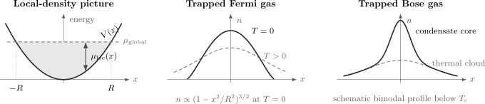
Harmonic trap with a local chemical potential and representative Fermi and Bose density profiles — The trap converts one global chemical potential into the spatially varying value $\mu_{\mathrm{loc}}=\mu_{\mathrm{global}}-V$ . In zero-temperature LDA, an ideal Fermi cloud has compact support and an inverted-power profile; a trapped Bose gas below its condensation crossover can display a narrow condensate contribution on a broader thermal cloud. The finite-temperature curves are schematic.

LDA conditions

LDA requires more than a large particle number. Check that:

the trap varies slowly over the local interparticle spacing or Fermi wavelength;
it varies slowly over the healing or correlation length when interactions matter;
the gas has reached local thermal and chemical equilibrium;
the observation probes scales larger than the level spacing and gradient region;
no tight direction that should remain quantized has been replaced by a continuum;
critical correlations have not grown to the trap-variation scale.

The approximation can fail near a cloud edge, a sharp interface, a very small trap, a critical region, or a rapidly varying optical structure.

Semiclassical Approximation Versus LDA

These terms are related but not identical.

The semiclassical trap approximation replaces discrete one-particle levels by a phase-space integral. It is a statement about spectral resolution.

The local-density approximation applies a homogeneous many-body equation of state at a position-dependent chemical potential. It is a statement about spatial scale separation.

For an ideal gas in a smooth potential, the two lead to the same phase-space expression:

n(\mathbf r) = g \int \frac{d^d p}{(2\pi\hbar)^d} \frac{1}{ e^{\beta[p^2/(2m)+V(\mathbf r)-\mu]} \mp1 },

where the upper minus sign is for bosons and the lower plus sign is for fermions.

For an interacting gas, LDA can remain useful even though the local equation of state is far from ideal. Conversely, a discrete noninteracting trap can be solved exactly without invoking LDA.

Three-Dimensional Local Profiles

Define the thermal wavelength

\lambda_T = \sqrt{ \frac{2\pi\hbar^2}{mk_{\mathrm B}T} }.

The local fugacity is

z(\mathbf r) = z_0e^{-\beta V(\mathbf r)},

where $z_0=e^{\beta\widetilde\mu}$ when the trap bottom and zero-point convention have been handled consistently.

For ideal bosons outside the condensate mode,

n_{\mathrm{th}}^{\mathrm B}(\mathbf r) = \frac{g}{\lambda_T^3} \operatorname{Li}_{3/2} \left[z(\mathbf r)\right].

For ideal fermions,

n^{\mathrm F}(\mathbf r) = \frac{g}{\lambda_T^3} \left[ -\operatorname{Li}_{3/2} \left[-z(\mathbf r)\right] \right].

In the dilute wings, $z(\mathbf r)\ll1$ , so both become

n(\mathbf r) \simeq \frac{g z_0}{\lambda_T^3} e^{-\beta V(\mathbf r)}.

For a harmonic trap, this is a Gaussian profile. The same cloud can therefore require quantum statistics near its center and Maxwell–Boltzmann statistics in its outer wings.

Trapped Ideal Bose Gas

For one ideal bosonic component, the ground orbital is

\phi_0(\mathbf r) = \prod_{a=1}^{3} \frac{1}{ \pi^{1/4}a_a^{1/2} } \exp \left( -\frac{x_a^2}{2a_a^2} \right).

If $N_0$ particles occupy that orbital, the condensate contribution is

n_0(\mathbf r) = N_0 \prod_{a=1}^{3} \frac{1}{\sqrt\pi a_a} \exp \left( -\frac{x_a^2}{a_a^2} \right).

The full ideal-gas density below the condensation crossover is

n(\mathbf r) = n_0(\mathbf r) + n_{\mathrm{th}}(\mathbf r).

This produces a bimodal spatial or velocity profile when the condensate is sufficiently resolved from the thermal cloud.

Condensation scale

At saturation, $z\to1$ and the semiclassical excited-state capacity is

N_{\mathrm{ex,max}} = \zeta(3) \left( \frac{k_{\mathrm B}T}{ \hbar\overline\omega } \right)^3

for a single component. The leading ideal critical scale is

k_{\mathrm B}T_c^{\mathrm{trap}} = \hbar\overline\omega \left[ \frac{N}{\zeta(3)} \right]^{1/3}.

Below this scale,

\frac{N_0}{N} \simeq 1- \left( \frac{T}{T_c^{\mathrm{trap}}} \right)^3

in the ideal semiclassical limit. The canonical derivation, finite-size qualifications, and dimensionality criterion are on Bose–Einstein Condensation.

Interaction warning

Repulsive interactions broaden the condensate beyond the oscillator ground state and can produce an interaction-dominated profile. The resulting Thomas–Fermi approximation is derived in Gross–Pitaevskii Equation; it is unrelated to Fermi–Dirac statistics despite the shared name.

Finite-temperature interactions also shift density profiles and the transition region. The ideal trapped gas is a benchmark, not a precision model for every condensate.

Trapped Ideal Fermi Gas at Zero Temperature

For $g$ equally populated, noninteracting internal components, fill trap levels up to a global Fermi excitation energy $E_{\mathrm F}^{\mathrm{trap}}$ . Semiclassical state counting gives

N = \frac{g}{6} \left( \frac{E_{\mathrm F}^{\mathrm{trap}}}{ \hbar\overline\omega } \right)^3.

Therefore

E_{\mathrm F}^{\mathrm{trap}} = \hbar\overline\omega \left( \frac{6N}{g} \right)^{1/3}.

Define the global trap Fermi temperature by

k_{\mathrm B}T_{\mathrm F}^{\mathrm{trap}} = E_{\mathrm F}^{\mathrm{trap}}.

This is not obtained from a volume-averaged density. It is the energy of the highest occupied trap shell measured from the trap bottom in the large- $N$ approximation.

Local Fermi scales

At $T=0$ , LDA gives the local Fermi energy

\epsilon_{\mathrm F}(\mathbf r) = E_{\mathrm F}^{\mathrm{trap}} - V_{\mathrm{ext}}(\mathbf r).

Where this quantity is positive,

k_{\mathrm F}(\mathbf r) = \frac{ \sqrt{2m\epsilon_{\mathrm F}(\mathbf r)} }{\hbar}

and

n(\mathbf r) = \frac{g}{6\pi^2} \left[ \frac{2m}{\hbar^2} \epsilon_{\mathrm F}(\mathbf r) \right]^{3/2}.

Outside the classically allowed ellipsoid, $n(\mathbf r)=0$ in the zero-temperature LDA.

Thomas–Fermi radii

Define

R_a = \sqrt{ \frac{ 2E_{\mathrm F}^{\mathrm{trap}} }{m\omega_a^2} }.

Then

n(\mathbf r) = n(\mathbf0) \left( 1- \sum_{a=1}^{3} \frac{x_a^2}{R_a^2} \right)^{3/2}

inside the ellipsoid, with

n(\mathbf0) = \frac{g}{6\pi^2} \left( \frac{ 2mE_{\mathrm F}^{\mathrm{trap}} }{\hbar^2} \right)^{3/2}.

Here Thomas–Fermi profile refers to the semiclassical filling of many trap states. It should not be confused with the interaction-dominated Thomas–Fermi condensate approximation.

Energetics of the Trapped Fermi Gas

With $D_{\mathrm{trap}}(E)\propto E^2$ , the zero-temperature excitation energy is

U_0-N\epsilon_0 = \frac{3}{4} N E_{\mathrm F}^{\mathrm{trap}},

where $\epsilon_0$ is the one-particle trap zero-point energy when absolute energies are retained.

For a harmonic potential, the virial theorem divides this excitation energy equally between kinetic and trapping contributions:

\langle K\rangle = \langle V\rangle = \frac{3}{8} N E_{\mathrm F}^{\mathrm{trap}}.

At low temperature and fixed $N$ , the trap density of states satisfies

D_{\mathrm{trap}} \left(E_{\mathrm F}^{\mathrm{trap}}\right) = \frac{3N}{ E_{\mathrm F}^{\mathrm{trap}} }.

The Sommerfeld Expansion then gives

\mu(T) = E_{\mathrm F}^{\mathrm{trap}} \left[ 1- \frac{\pi^2}{3} \left( \frac{T}{T_{\mathrm F}^{\mathrm{trap}}} \right)^2 + O \left( \frac{T^4}{(T_{\mathrm F}^{\mathrm{trap}})^4} \right) \right]

and

C_{V,N} = \pi^2Nk_{\mathrm B} \frac{T}{T_{\mathrm F}^{\mathrm{trap}}} + O \left[ Nk_{\mathrm B} \frac{T^3}{(T_{\mathrm F}^{\mathrm{trap}})^3} \right].

The coefficient differs from the uniform three-dimensional gas because the trap density of states has a different energy dependence.

Hydrostatic Balance and Equation-of-State Mapping

At uniform temperature, LDA implies

dP = n\,d\mu.

Taking a spatial gradient and using $\nabla\mu_{\mathrm{loc}}=-\nabla V$ gives

\nabla P(\mathbf r) = -n(\mathbf r) \nabla V_{\mathrm{ext}}(\mathbf r).

This is hydrostatic force balance. It makes trapped profiles useful rather than merely inconvenient: a single image samples the homogeneous equation of state over a range of $\mu_{\mathrm{loc}}$ .

If $V(\mathbf r)$ and the imaging geometry are calibrated, measured density profiles can be transformed into pressure, compressibility, and other local thermodynamic quantities. Such inversions require symmetry assumptions, finite-resolution corrections, and a reliable relationship between optical signal and atom number.

Trap Thermodynamic Limit

A finite harmonic trap has a discrete spectrum and finite particle number, so its partition function is analytic. A sharp thermodynamic transition requires a trap thermodynamic limit.

In $d$ dimensions, take

N\to\infty, \qquad \overline\omega\to0,

while keeping

N\overline\omega^d

fixed. This keeps characteristic density and degeneracy scales finite while the level spacing vanishes.

For a real finite cloud:

condensation and degeneracy onsets are rounded;
shell effects can survive at small $N$ or low $T$ ;
critical temperatures acquire finite-size and interaction shifts;
the precise crossover criterion depends on the observable.

The Thermodynamic Limit page owns the general limiting logic. Finite-Size Effects provides the cross-system audit of shell resolution, finite- $N$ rounding, correlation lengths, and experimental resolution; this page retains the trap-specific derivations.

Anisotropy and Dimensional Crossover

Strong confinement can freeze one or two oscillator directions. If

k_{\mathrm B}T, \quad \mu_{\mathrm{int}}, \quad E_{\mathrm F} \ll \hbar\omega_{\perp},

then excitations in the tight direction are suppressed and the gas becomes effectively lower dimensional.

One must retain the discrete ground state in each frozen direction and integrate only over the weakly confined directions. Replacing every direction by a three-dimensional continuum can produce wrong densities of states, couplings, and transition criteria.

Low-Dimensional Quantum Gases owns the general dimensionality analysis and explains why quasi-one-dimensional and quasi-two-dimensional interaction parameters require confinement-induced renormalization beyond ideal state counting.

From Density to Images

Cold-atom experiments commonly use two broad measurement geometries.

In-situ imaging

An absorption or phase-contrast image usually yields a line-of-sight column density:

n_{\mathrm{col}}(x,z) = \int dy\, n(x,y,z),

after optical calibration. Reconstructing the three-dimensional density may require cylindrical or spherical symmetry, tomographic data, or a model fit.

Time-of-flight expansion

After the trap is released, a sufficiently long collisionless ballistic expansion approximately maps initial momentum to position:

\mathbf r(t) \simeq \frac{\mathbf p}{m}t.

This relation is not automatic. Mean-field release energy, collisions, hydrodynamic flow, finite expansion time, gravity, and switching dynamics can alter the mapping.

For a condensate, anisotropic expansion can reflect interaction and confinement energy. For a degenerate Fermi gas, cloud size and shape can reveal Fermi pressure, but an interacting cloud requires the appropriate dynamical model.

Experimental Signatures

Bosons

The 1995 dilute-gas Bose–Einstein condensation experiments used trapped alkali atoms, evaporative cooling, and spatial or velocity-distribution signatures. A characteristic observation was the emergence of a narrow, nonthermal component on a broad thermal distribution.

That bimodality is strong evidence when the imaging response, expansion dynamics, and interaction model are controlled. It should not be reduced to the statement that every atom occupies one point in momentum space; the condensate occupies a trap orbital with finite spatial and momentum widths.

Fermions

The onset of Fermi degeneracy was observed in trapped potassium-40 in 1999. Unlike a Bose condensate, an ideal Fermi gas does not develop a macroscopically occupied one-particle orbital. Signatures include:

saturation of low-energy state occupation;
a cloud size supported by Fermi pressure;
deviations from a classical Gaussian profile;
Pauli suppression of collisions and fluctuations;
thermometry expressed through $T/T_{\mathrm F}^{\mathrm{trap}}$ .

Mixtures of internal states are often needed for efficient $s$ -wave thermalization, because identical spin-polarized fermions suppress that channel at ultralow energy. The component populations then enter $g$ , the Fermi scales, and interaction physics explicitly.

A Practical Analysis Workflow

Specify the trap potential and energy zero.
Decide whether exact discrete levels, a semiclassical integral, or LDA is controlled.
Keep internal components and their chemical potentials explicit.
For bosons, separate the lowest mode before taking a continuum limit.
For fermions, distinguish the global trap Fermi energy from local density-based Fermi energies.
Solve the number equation using the actual trap density of states.
Predict the three-dimensional density or momentum distribution.
Map that distribution through the measurement protocol to the recorded column image.
Check finite size, interactions, anisotropy, and expansion dynamics before comparing with data.

Common Mistakes

Using a box formula with an average trap density.
The harmonic trap has $D(E)\propto E^2$ , not the uniform three-dimensional $D(E)\propto E^{1/2}$ .

Calling $E_{\mathrm F}^{\mathrm{trap}}$ a local Fermi energy everywhere.
It is a global shell-filling scale. The local value decreases as $E_{\mathrm F}^{\mathrm{trap}}-V(\mathbf r)$ .

Dropping the zero-point convention.
For bosons, $\mu\le\epsilon_0$ in absolute energies, while $\widetilde\mu\le0$ after shifting the trap bottom.

Replacing the condensate mode by a continuum integral.
That removes the very mode whose macroscopic occupation defines ideal-gas condensation.

Treating LDA as exact.
Gradient, finite-size, shell, edge, and critical-correlation effects can invalidate it.

Equating semiclassical state counting with classical statistics.
A phase-space integral can still carry fully quantum Bose or Fermi occupation factors.

Using three-dimensional formulas in a frozen anisotropic trap.
Tightly confined directions remain discrete and change both state counting and interactions.

Counting spin degeneracy twice.
Either include $g$ in the density of states or sum over components explicitly.

Interpreting every time-of-flight image as a momentum distribution.
The mapping requires ballistic expansion and controlled release dynamics.

Calling every finite-cloud crossover a phase transition.
Exact nonanalyticity requires an appropriate thermodynamic limit.

Confusing two Thomas–Fermi approximations.
Semiclassical Fermi filling and interaction-dominated condensate profiles arise from different physics.

Canonical Boundaries and Connections

Bose Gas Formula Sheet collects the leading homogeneous and harmonic-trap ideal-gas formulas for rapid lookup.
Quantum Harmonic Oscillator owns the one-particle oscillator spectrum and wavefunctions.
Bose–Einstein Condensation owns the general condensation criterion, trapped critical temperature, condensate fraction, finite-size qualifications, and coherence interpretation.
Ideal Bose Gas and Ideal Fermi Gas own the uniform benchmark models.
Fermi Momentum and Fermi Energy owns uniform and local continuum Fermi-scale conventions.
Sommerfeld Expansion owns the low-temperature asymptotic method.
Maxwell–Boltzmann Limit owns the classical trap wings and dilute criterion.
Chemical Potential owns the general local-equilibrium relation in an external potential.
Gross–Pitaevskii Equation owns interacting condensate profiles, collective dynamics, vortices, and the condensate Thomas–Fermi limit.
Low-Dimensional Quantum Gases owns effective one- and two-dimensional thermodynamics and fluctuation constraints.
AMO platform pages own trap implementation, atom preparation, laser control, species-specific spectroscopy, and experimental uncertainty budgets.

References

C. J. Pethick and H. Smith, Bose–Einstein Condensation in Dilute Gases, 2nd ed., Cambridge University Press (2008) — trapped Bose gases, semiclassical profiles, interactions, and experiments.
L. Pitaevskii and S. Stringari, Bose–Einstein Condensation and Superfluidity, Oxford University Press (2016) — equilibrium and dynamical theory of trapped quantum gases.
F. Dalfovo, S. Giorgini, L. P. Pitaevskii, and S. Stringari, “Theory of Bose–Einstein Condensation in Trapped Gases”, Reviews of Modern Physics 71, 463–512 (1999) — authoritative review of trapped dilute Bose gases.
S. Giorgini, L. P. Pitaevskii, and S. Stringari, “Theory of Ultracold Atomic Fermi Gases”, Reviews of Modern Physics 80, 1215–1274 (2008) — trapped and uniform Fermi gases, interactions, profiles, and thermodynamics.
W. Ketterle and N. J. van Druten, “Bose–Einstein Condensation of a Finite Number of Particles Trapped in One or Three Dimensions”, Physical Review A 54, 656–660 (1996) — finite-size and trap-dimensionality analysis.
M. H. Anderson, J. R. Ensher, M. R. Matthews, C. E. Wieman, and E. A. Cornell, “Observation of Bose–Einstein Condensation in a Dilute Atomic Vapor”, Science 269, 198–201 (1995) — trapped rubidium-87 condensation and its velocity-distribution signatures.
K. B. Davis, M.-O. Mewes, M. R. Andrews, N. J. van Druten, D. S. Durfee, D. M. Kurn, and W. Ketterle, “Bose–Einstein Condensation in a Gas of Sodium Atoms”, Physical Review Letters 75, 3969–3973 (1995) — trapped sodium condensation and bimodal expansion profiles.
B. DeMarco and D. S. Jin, “Onset of Fermi Degeneracy in a Trapped Atomic Gas”, Science 285, 1703–1706 (1999) — first degenerate trapped atomic Fermi gas.
A. G. Truscott, K. E. Strecker, W. I. McAlexander, G. B. Partridge, and R. G. Hulet, “Observation of Fermi Pressure in a Gas of Trapped Atoms”, Science 291, 2570–2572 (2001) — trap-size manifestation of Fermi pressure.

Exercises

Count isotropic oscillator shells

For a three-dimensional isotropic harmonic oscillator, show that shell $q=n_x+n_y+n_z$ has degeneracy

d_q = \frac{(q+1)(q+2)}{2}

and that the number of orbitals through shell $q$ is

\mathcal N_q = \frac{(q+1)(q+2)(q+3)}{6}.

Solution

The degeneracy is the number of nonnegative integer solutions of

n_x+n_y+n_z = q.

By stars and bars,

d_q = \binom{q+2}{2} = \frac{(q+1)(q+2)}{2}.

Summing the shells and using the hockey-stick identity gives

\begin{aligned} \mathcal N_q &= \sum_{j=0}^{q} \binom{j+2}{2} \\ &= \binom{q+3}{3} \\ &= \frac{(q+1)(q+2)(q+3)}{6}. \end{aligned}

Derive the harmonic-trap density of states

For an anisotropic harmonic trap in $d$ dimensions, derive the leading semiclassical cumulative state count and density of states.

Solution

At large quantum numbers, count the volume in the nonnegative region satisfying

\sum_{a=1}^{d} \hbar\omega_a n_a \le E.

Define

y_a = \frac{\hbar\omega_a n_a}{E}.

The unit simplex $\sum_a y_a\le1$ has volume $1/d!$ . The Jacobian is

\prod_a dn_a = \frac{E^d}{ \hbar^d\prod_a\omega_a } \prod_a dy_a.

Therefore

\mathcal N(E) \simeq \frac{E^d}{ d!\hbar^d\prod_a\omega_a }.

Differentiating gives

D(E) \simeq \frac{E^{d-1}}{ (d-1)!\hbar^d\prod_a\omega_a }.

Recover the classical Gaussian cloud

Use the Maxwell–Boltzmann phase-space distribution in a harmonic trap to derive the spatial density and its root-mean-square width in direction $a$ .

Solution

In the dilute limit,

n(\mathbf r) \propto e^{-\beta V(\mathbf r)}.

For the harmonic potential,

n(\mathbf r) = n(\mathbf0) \prod_a \exp \left( -\frac{ m\omega_a^2x_a^2 }{2k_{\mathrm B}T} \right).

Comparing each factor with a normalized Gaussian gives

\langle x_a^2\rangle = \frac{k_{\mathrm B}T}{m\omega_a^2}.

Thus the root-mean-square width is

\sigma_a = \sqrt{ \frac{k_{\mathrm B}T}{m\omega_a^2} }.

Derive the ideal trapped-boson critical scale

For one bosonic component in a three-dimensional harmonic trap, derive $T_c^{\mathrm{trap}}$ and the leading condensate fraction from the semiclassical density of states.

Solution

At saturation, $z\to1$ and

\begin{aligned} N_{\mathrm{ex,max}} &= \frac{1}{2(\hbar\overline\omega)^3} \int_0^{\infty} dE\, \frac{E^2}{e^{\beta E}-1} \\ &= \zeta(3) \left( \frac{k_{\mathrm B}T}{ \hbar\overline\omega } \right)^3. \end{aligned}

Setting $N=N_{\mathrm{ex,max}}(T_c)$ gives

k_{\mathrm B}T_c^{\mathrm{trap}} = \hbar\overline\omega \left[ \frac{N}{\zeta(3)} \right]^{1/3}.

Below $T_c$ , the excited population scales as $T^3$ , so

\frac{N_0}{N} = 1- \left( \frac{T}{T_c^{\mathrm{trap}}} \right)^3.

Finite size and interactions modify this leading ideal result.

Derive the trap Fermi energy

For total particle number $N$ distributed equally among $g$ ideal fermion components, derive the global trap Fermi energy. Compare it with exact shell counting in an isotropic trap.

Solution

The semiclassical cumulative number is

N = g \frac{(E_{\mathrm F}^{\mathrm{trap}})^3}{ 6(\hbar\overline\omega)^3 }.

Solving gives

E_{\mathrm F}^{\mathrm{trap}} = \hbar\overline\omega \left( \frac{6N}{g} \right)^{1/3}.

For an isotropic trap with all shells through $q_{\mathrm F}$ filled,

N = g \frac{ (q_{\mathrm F}+1) (q_{\mathrm F}+2) (q_{\mathrm F}+3) }{6}.

At large $q_{\mathrm F}$ ,

N \simeq g\frac{q_{\mathrm F}^3}{6},

so $q_{\mathrm F}\hbar\omega$ approaches the semiclassical result. The exact expression retains shell and zero-point corrections.

Normalize the zero-temperature Fermi profile

Show that

n(\mathbf r) = n(\mathbf0) \left( 1- \sum_a\frac{x_a^2}{R_a^2} \right)^{3/2}

integrates to

N = \frac{g}{6} \left( \frac{E_{\mathrm F}^{\mathrm{trap}}}{ \hbar\overline\omega } \right)^3.

Solution

Set $u_a=x_a/R_a$ . Then

d^3r = R_xR_yR_z\,d^3u,

and the support is the unit ball. The dimensionless integral is

\int_{u<1} d^3u\, (1-u^2)^{3/2} = \frac{\pi^2}{8}.

Also,

R_xR_yR_z = \frac{1}{ \omega_x\omega_y\omega_z } \left( \frac{2E_{\mathrm F}^{\mathrm{trap}}}{m} \right)^{3/2}.

Multiplying by

n(\mathbf0) = \frac{g}{6\pi^2} \left( \frac{2mE_{\mathrm F}^{\mathrm{trap}}}{\hbar^2} \right)^{3/2}

gives

N = \frac{g}{6} \frac{(E_{\mathrm F}^{\mathrm{trap}})^3}{ \hbar^3\omega_x\omega_y\omega_z }.

Since $\overline\omega^3=\omega_x\omega_y\omega_z$ , this is the required result.

Obtain the low-temperature Fermi heat capacity

Use the trap density of states and the Sommerfeld expansion to derive the leading fixed- $N$ heat capacity.

Solution

For total density of states

D(E) = \frac{gE^2}{ 2(\hbar\overline\omega)^3 },

the zero-temperature number is

N = \frac{gE_{\mathrm F}^3}{ 6(\hbar\overline\omega)^3 }.

Therefore

D(E_{\mathrm F}) = \frac{3N}{E_{\mathrm F}}.

The general fixed-number Sommerfeld result is

C_{V,N} = \frac{\pi^2}{3} D(E_{\mathrm F}) k_{\mathrm B}^2T.

Substitution yields

C_{V,N} = \pi^2Nk_{\mathrm B} \frac{T}{T_{\mathrm F}^{\mathrm{trap}}}.

Project a Fermi cloud into a column density

For the zero-temperature profile, integrate along $y$ and show that the column density has exponent $2$ rather than $3/2$ .

Solution

At fixed $x,z$ , define

A = 1- \frac{x^2}{R_x^2} - \frac{z^2}{R_z^2}.

The allowed line of sight satisfies

|y| \le R_y\sqrt A.

Then

\begin{aligned} n_{\mathrm{col}}(x,z) &= n(\mathbf0) \int_{-R_y\sqrt A}^{R_y\sqrt A} dy\, \left( A- \frac{y^2}{R_y^2} \right)^{3/2} \\ &= n(\mathbf0)R_yA^2 \int_{-1}^{1} dt\, (1-t^2)^{3/2}. \end{aligned}

The remaining integral is $3\pi/8$ , so

n_{\mathrm{col}}(x,z) = \frac{3\pi}{8} n(\mathbf0)R_y \left( 1- \frac{x^2}{R_x^2} - \frac{z^2}{R_z^2} \right)^2.

This illustrates why a recorded column profile does not have the same exponent as the underlying three-dimensional density.