Bose–Einstein Statistics

Bose–Einstein statistics gives the equilibrium occupation of ideal bosonic modes. For a mode $i$ with one-particle energy $\epsilon_i$,

$$\overline n_i = \frac{1}{ e^{\beta(\epsilon_i-\mu)}-1 }, \qquad \beta = \frac{1}{k_{\mathrm B}T}.$$

The minus sign in the denominator is not a convention. It follows from the unrestricted bosonic occupation numbers

$$n_i = 0,1,2,\ldots.$$

For the ordinary grand-canonical sum to converge, every included mode must satisfy

$$\epsilon_i-\mu > 0.$$

In particular, for a finite ideal system with lowest one-particle energy $\epsilon_0$,

$$\mu < \epsilon_0.$$

This page owns the derivation, interpretation, fluctuations, and limiting behavior of the Bose–Einstein occupation law. The formula card is the compact lookup entry; exchange symmetry itself belongs to Bosons.

Assumptions

The standard formula requires more than the statement that the particles are bosons. Its direct derivation assumes:

• thermal equilibrium at temperature $T$;
• a grand-canonical description with chemical potential $\mu$;
• independent bosonic modes, or quasiparticle modes described by a diagonal quadratic Hamiltonian;
• well-defined one-mode energies $\epsilon_i$;
• unrestricted occupations $n_i=0,1,2,\ldots$;
• convergence of every bosonic geometric series.

For ideal modes,

$$H = \sum_i \epsilon_i n_i, \qquad N = \sum_i n_i.$$

The formula can remain useful for weakly interacting quasiparticles after a controlled diagonalization, but it is not automatically exact for interacting particles, driven systems, or arbitrary nonequilibrium states.

From Exchange Symmetry to Thermodynamics

Bosonic exchange symmetry says that identical-particle states are symmetric under particle exchange. In occupation language, that permits any nonnegative integer number of bosons in one mode.

That kinematic statement does not by itself determine a thermal distribution. Bose–Einstein statistics appears only after combining:

$$\begin{gathered} \text{bosonic occupations} \\ +\ \text{equilibrium weights} \\ +\ \text{an ensemble constraint}. \end{gathered}$$

The separation matters. A pure number state, a coherent state, a squeezed state, and a thermal state may all describe bosonic modes, but only the thermal state has the Bose–Einstein geometric occupation distribution derived below.

Grand-Canonical Derivation

Introduce the grand Hamiltonian

$$K = H-\mu N.$$

For independent modes,

$$K = \sum_i (\epsilon_i-\mu)n_i.$$

Because the mode number operators commute, the grand partition function factorizes:

$$\Xi = \prod_i \xi_i.$$

For one bosonic mode,

$$\begin{aligned} \xi_i &= \sum_{n_i=0}^{\infty} e^{-\beta(\epsilon_i-\mu)n_i} \\ &= \sum_{n_i=0}^{\infty} q_i^{n_i}, \end{aligned}$$

where

$$q_i \equiv e^{-\beta(\epsilon_i-\mu)}.$$

If $0\leq q_i<1$, the geometric series gives

$$\xi_i = \frac{1}{1-q_i}.$$

The mean occupation follows from a logarithmic derivative:

$$\begin{aligned} \overline n_i &= q_i \frac{\partial}{\partial q_i} \ln\xi_i \\ &= \frac{q_i}{1-q_i}. \end{aligned}$$

Substituting the definition of $q_i$ yields

$$\overline n_i = \frac{1}{ e^{\beta(\epsilon_i-\mu)}-1 }.$$

The full ideal-mode grand potential is therefore

$$\Omega_{\mathrm G} = k_{\mathrm B}T \sum_i \ln \left[ 1-e^{-\beta(\epsilon_i-\mu)} \right].$$

Thermodynamic sums over $\overline n_i$ follow by differentiating this potential or by summing the mode occupations directly.

The Full One-Mode Distribution

The Bose–Einstein formula is a mean. The complete probability distribution for one ideal thermal mode is

$$P_i(n) = (1-q_i)q_i^n, \qquad n=0,1,2,\ldots.$$

Normalization follows from

$$\sum_{n=0}^{\infty} P_i(n) = (1-q_i) \sum_{n=0}^{\infty} q_i^n = 1.$$

Successive probabilities obey

$$\frac{P_i(n+1)}{P_i(n)} = q_i = e^{-\beta(\epsilon_i-\mu)}.$$

The distribution is geometric, not Poissonian. Expressed in terms of the mean,

$$q_i = \frac{\overline n_i}{1+\overline n_i},$$

so

$$P_i(n) = \frac{1}{1+\overline n_i} \left( \frac{\overline n_i}{1+\overline n_i} \right)^n.$$

Dimensionless Form

Define the dimensionless distance above the chemical potential,

$$x \equiv \beta(\epsilon-\mu).$$

The Bose function is

$$f_{\mathrm B}(x) = \frac{1}{e^x-1}, \qquad x>0.$$

Its entire shape is controlled by one variable. Large positive $x$ gives dilute classical occupation, while $x\to0^+$ produces large occupation and enhanced fluctuations.

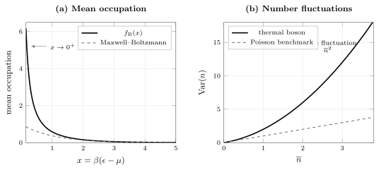
The Bose–Einstein occupation $f_{\mathrm B}(x)$ exceeds the Maxwell–Boltzmann approximation and diverges as $x=\beta(\epsilon-\mu)\to0^+$. A thermal bosonic mode has $\operatorname{Var}(n)=\overline n(1+\overline n)$, larger than the Poisson benchmark $\operatorname{Var}(n)=\overline n$.

Occupation Enhancement

The geometric series can be expanded as

$$\overline n_i = q_i + q_i^2 + q_i^3 + \cdots.$$

The first term is the Maxwell–Boltzmann occupation. The positive higher powers are the equilibrium statistical correction associated with unrestricted bosonic occupation.

The same enhancement appears algebraically in creation-operator matrix elements:

$$a_i^\dagger \lvert n_i\rangle = \sqrt{n_i+1} \lvert n_i+1\rangle.$$

Transition probabilities generated by a linear creation operator therefore contain a factor $n_i+1$. This is often called Bose enhancement or stimulated emission.

The two statements are related by bosonic occupation algebra, but they answer different questions. The Bose–Einstein distribution is an equilibrium probability law; the factor $n+1$ in a transition rate is a dynamical matrix-element effect.

Fluctuations and Bunching

For the geometric distribution,

$$\langle n_i^2\rangle = \overline n_i + 2\overline n_i^2.$$

Hence

$$\operatorname{Var}(n_i) = \overline n_i \left( 1+\overline n_i \right).$$

The first term is the Poisson-like contribution. The second is the bosonic excess fluctuation.

The normally ordered second moment is

$$\langle n_i(n_i-1)\rangle = 2\overline n_i^2.$$

For one ideal thermal mode with nonzero mean, the normalized equal-time second-order coherence is

$$g^{(2)}(0) \equiv \frac{ \langle n_i(n_i-1)\rangle }{ \overline n_i^2 } = 2.$$

This is the ideal single-mode thermal bunching result. Multimode detection, finite time resolution, interactions, coherence, and detector response can change the observed value, so $g^{(2)}(0)=2$ is not a universal statement about every bosonic source.

The relative fluctuation is

$$\frac{ \sqrt{\operatorname{Var}(n_i)} }{ \overline n_i } = \sqrt{ 1+ \frac{1}{\overline n_i} }.$$

It approaches one, rather than zero, when one ideal thermal mode becomes highly occupied. Bulk thermodynamic relative fluctuations can still vanish after many modes or spatial cells are combined. A macroscopically occupied condensate mode requires special ensemble and interaction care.

Fluctuation–Response Identity

Differentiate the occupation with respect to chemical potential:

$$\left( \frac{\partial\overline n_i}{\partial\mu} \right)_T = \beta \overline n_i \left( 1+\overline n_i \right).$$

Therefore

$$\left( \frac{\partial\overline n_i}{\partial\mu} \right)_T = \beta \operatorname{Var}(n_i).$$

Similarly,

$$- \frac{1}{\beta} \left( \frac{\partial\overline n_i}{\partial\epsilon_i} \right)_{T,\mu} = \operatorname{Var}(n_i).$$

The sharp growth of occupation near $\epsilon_i=\mu$ is inseparable from enhanced mode-number fluctuations in the ideal grand-canonical description.

Chemical-Potential Constraint

The one-mode sum converges only when

$$q_i = e^{-\beta(\epsilon_i-\mu)} < 1.$$

At positive temperature this is equivalent to

$$\mu < \epsilon_i.$$

The strictest condition comes from the lowest mode:

$$\mu < \epsilon_0.$$

If the energy zero is chosen so that $\epsilon_0=0$, then

$$\mu < 0$$

for a finite ideal Bose system described by the unconstrained grand-canonical sum.

The inequality concerns the relative energy convention. Under the joint shift

$$\epsilon_i' = \epsilon_i+C, \qquad \mu' = \mu+C,$$

the difference $\epsilon_i-\mu$ and every occupation remain unchanged.

Approach to the Lowest Mode

Let

$$\delta \equiv \epsilon_0-\mu > 0.$$

Then

$$\overline n_0 = \frac{1}{e^{\beta\delta}-1}.$$

For $\beta\delta\ll1$,

$$\overline n_0 \sim \frac{1}{\beta\delta}.$$

The divergence signals that the lowest mode cannot always be treated as an ordinary thermodynamic correction. In a fixed-density ideal Bose gas, the chemical potential approaches $\epsilon_0$ from below and the ground-state occupation may become macroscopic.

That statement is a bridge to the ideal Bose gas and Bose–Einstein condensation. Whether condensation occurs, and how the excited-state population saturates, depends on the density of states, dimensionality, confinement, and thermodynamic limit.

Conserved and Nonconserved Boson Number

For atoms in a sealed or effectively number-conserving system, $\mu$ is adjusted so that

$$\overline N = \sum_i \overline n_i$$

matches the required mean particle number.

For equilibrium excitations whose number is not conserved, the associated chemical potential is ordinarily zero. Important examples are photons in blackbody equilibrium and phonons in a crystal:

$$\mu_\gamma = 0, \qquad \mu_{\mathrm{ph}} = 0.$$

This is not a statement that every bosonic species has zero chemical potential. Conserved atoms generally have nonzero $\mu$, and driven or approximately conserved quasiparticle populations can sometimes be described by an effective chemical potential. Such a parameter must be justified by conservation laws and timescales.

High-Energy and Dilute Limit

When

$$x = \beta(\epsilon-\mu) \gg 1,$$

the occupation is small. Writing $y=e^{-x}$ gives

$$\begin{aligned} f_{\mathrm B}(x) &= \frac{y}{1-y} \\ &= y+y^2+y^3+\cdots. \end{aligned}$$

Therefore

$$f_{\mathrm B}(x) \simeq e^{-x}.$$

This is the Maxwell–Boltzmann limit. Classical Limit of Quantum Statistics turns this mode-level expansion into the homogeneous criterion $n\lambda_T^d/g\ll1$ and derives the unified Bose/Fermi virial correction. The leading relative correction here is of order $e^{-x}$:

$$\frac{ f_{\mathrm B}(x)-e^{-x} }{ e^{-x} } = e^{-x} + O(e^{-2x}).$$

Quantum statistics becomes negligible mode by mode when every relevant occupation is much less than one. In a gas, that condition is commonly expressed through low fugacity or a small phase-space density.

Highly Occupied Limit

For $x\ll1$ with $x>0$,

$$\frac{1}{e^x-1} = \frac{1}{x} - \frac{1}{2} + \frac{x}{12} - \frac{x^3}{720} + O(x^5).$$

The leading term is

$$\overline n \simeq \frac{k_{\mathrm B}T}{\epsilon-\mu}.$$

This is the classical-field or Rayleigh–Jeans form for a highly occupied mode. Applying it to arbitrarily high energies produces ultraviolet divergences; the full Bose–Einstein denominator supplies the quantum suppression at large $x$.

Zero-Temperature Limit

At fixed $\mu<\epsilon_0$,

$$\lim_{T\to0^+} \overline n_i = 0$$

for every included mode.

That limit is not the correct fixed-particle-number limit for a Bose gas with particles present. At fixed $N$, the chemical potential generally changes with temperature and can approach the lowest one-particle energy. The ground mode must then be separated from the excited-state continuum.

The lesson is simple: a temperature limit is incomplete unless one states which thermodynamic variables are held fixed.

Mode Versus Degenerate Level

The Bose–Einstein formula gives occupation per mode. If an energy level $\epsilon$ has degeneracy $g_\epsilon$ and the modes are independent, then

$$\overline N_\epsilon = g_\epsilon f_{\mathrm B} \left[ \beta(\epsilon-\mu) \right].$$

The level variance is

$$\operatorname{Var}(N_\epsilon) = g_\epsilon \overline n_\epsilon \left( 1+\overline n_\epsilon \right)$$

when the degenerate modes fluctuate independently.

In a continuum approximation, sums become integrals over the one-particle density of states $g(\epsilon)$:

$$\overline N = \int d\epsilon\, g(\epsilon) \frac{1}{ e^{\beta(\epsilon-\mu)}-1 }.$$

The density of states controls whether the excited modes can hold an arbitrarily large density. This is where dimensionality enters the theory of ideal-gas condensation.

Entropy Per Mode

For a geometric thermal mode, the von Neumann entropy can be written entirely in terms of $\overline n$:

$$\frac{s_{\mathrm B}}{k_{\mathrm B}} = \left( 1+\overline n \right) \ln \left( 1+\overline n \right) - \overline n \ln\overline n.$$

This expression follows by substituting the geometric probabilities into

$$s = -k_{\mathrm B} \sum_n P(n)\ln P(n).$$

It vanishes as $\overline n\to0$ and grows logarithmically for large occupation. Summing it over independent modes gives the entropy of an ideal bosonic gas or a collection of independent thermal oscillators.

Example: One Harmonic-Oscillator Mode

For one oscillator of angular frequency $\omega$,

$$H = \hbar\omega \left( n+\frac{1}{2} \right).$$

If oscillator quanta are not conserved, $\mu=0$. The mean excitation number is

$$\overline n = \frac{1}{e^{\beta\hbar\omega}-1}.$$

The mean energy is

$$U = \hbar\omega \left( \overline n+\frac{1}{2} \right).$$

The zero-point term does not affect the normalized occupation probabilities. The heat capacity is

$$C = k_{\mathrm B} (\beta\hbar\omega)^2 \frac{ e^{\beta\hbar\omega} }{ \left( e^{\beta\hbar\omega}-1 \right)^2 }.$$

At high temperature, $U-\hbar\omega/2$ approaches $k_{\mathrm B}T$. At low temperature, thermal excitation is exponentially suppressed.

Example: Photons

Each electromagnetic normal mode is a bosonic oscillator. In blackbody equilibrium, photon number is not conserved, so

$$\mu_\gamma = 0.$$

For a mode with angular frequency $\omega$,

$$\overline n_\omega = \frac{1}{e^{\beta\hbar\omega}-1}.$$

Multiplying the mean energy per mode by the electromagnetic density of states and polarization degeneracy produces Planck’s radiation law. The spectral derivation and historical evidence belong to Planck’s Radiation Law.

Example: Phonons

In a harmonic crystal, each normal mode with branch label $s$ and wavevector $\mathbf k$ has mean occupation

$$\overline n_{\mathbf k s} = \frac{1}{ e^{\beta\hbar\omega_{\mathbf k s}}-1 }.$$

Equilibrium phonon number is not conserved, so the phonon chemical potential is zero. Summing $\hbar\omega_{\mathbf k s}\overline n_{\mathbf k s}$ over the phonon density of states gives the thermal lattice energy in the harmonic approximation. Phonons as Many-Body Excitations derives the modes, operators, zero-point term, and displacement correlations behind this statistical description.

The low-temperature power law depends on the acoustic dispersion and spatial dimension; the high-temperature limit approaches classical equipartition over thermally accessible modes.

Example: Conserved Bosonic Atoms

For a dilute ideal gas of bosonic atoms, particle number is conserved on the equilibrium timescale. The chemical potential is fixed by

$$N = \sum_i \frac{1}{ e^{\beta(\epsilon_i-\mu)}-1 }.$$

As the gas is cooled at fixed density, $\mu$ rises toward $\epsilon_0$. If the excited-state sum has a finite maximum at $\mu=\epsilon_0$, additional particles accumulate in the lowest mode in the thermodynamic limit.

This mechanism is Bose–Einstein condensation in the ideal model. Interactions, trapping geometry, finite size, dimensionality, and experimental preparation determine how the ideal result must be modified.

Interactions and Quasiparticles

For interacting bosons, the microscopic Hamiltonian need not be diagonal in the original occupation numbers. Then

$$H \neq \sum_i \epsilon_i n_i$$

in the basis of bare one-particle modes, and the independent geometric-mode derivation fails.

A quadratic effective Hamiltonian may sometimes be diagonalized into bosonic quasiparticles:

$$H_{\mathrm{eff}} = E_0 + \sum_\alpha E_\alpha b_\alpha^\dagger b_\alpha.$$

If those quasiparticles equilibrate and their number is not conserved, then

$$\overline n_\alpha = \frac{1}{e^{\beta E_\alpha}-1}.$$

This does not mean the original particle occupations have the same simple distribution. One must identify which modes diagonalize the effective theory and which conserved charges determine their chemical potentials.

Finite Systems and the Thermodynamic Limit

For a finite ideal system, the convergence condition is strict:

$$\mu < \epsilon_0.$$

All occupations are finite for finite $T$ and finite separation $\epsilon_0-\mu$.

A sharp condensation transition is a thermodynamic-limit statement. In a finite trap or box, observables vary smoothly and the lowest-mode occupation can become large without a mathematical nonanalyticity.

Grand-canonical fluctuations of an ideal condensate can also be anomalously large. Fixed-$N$ constraints and interactions alter those fluctuations. The Bose–Einstein mean occupation remains the correct excited-mode building block in its regime, but ensemble-dependent condensate fluctuations should not be inferred from it without further analysis.

Canonical Boundaries

This page owns:

• the grand-canonical derivation of the Bose–Einstein occupation factor;
• the geometric one-mode probability distribution;
• occupation enhancement, variance, and ideal thermal bunching;
• the chemical-potential convergence condition;
• dilute, highly occupied, and zero-temperature limits;
• mode-level examples for oscillators, photons, phonons, and conserved atoms.

Other pages own:

• symmetrization and the definition of bosons: Composite Systems and Entanglement;
• the general Fock-space trace and number-sector statistics: Grand-Canonical Ensemble;
• the shared dilute criterion and exchange-cycle expansion: Classical Limit of Quantum Statistics;
• conserved-number, interacting-system, and sign-convention meanings of chemical potential: Chemical Potential;
• the compact expression for quick lookup: Reference;
• density-of-states thermodynamics and condensation criteria: Ideal Bose Gas and Bose–Einstein Condensation;
• detailed photon spectra and historical evidence: Experiments and Historical Development;
• interacting Bose gases and Bogoliubov quasiparticles: Interacting Systems and Approximation Methods.

Common Mistakes

• Treating Bose–Einstein statistics as a consequence of indistinguishability alone, without equilibrium assumptions.
• Forgetting that the formula gives a mean occupation, not an allowed eigenvalue.
• Replacing the geometric one-mode distribution by a Poisson distribution.
• Allowing $\mu\geq\epsilon_0$ in the ordinary ideal grand-canonical sum.
• Setting $\mu=0$ for every kind of boson.
• Calling $\mu$ a one-particle energy rather than a thermodynamic control parameter.
• Confusing a highly occupied thermal mode with a coherent state.
• Assuming $g^{(2)}(0)=2$ for arbitrary multimode, interacting, or coherently driven bosonic fields.
• Applying the Rayleigh–Jeans approximation at arbitrarily high energy.
• Taking $T\to0$ at fixed $\mu<\epsilon_0$ and calling the result the fixed-$N$ ground state.
• Using the per-mode formula as though it already included level degeneracy or density of states.
• Applying independent-mode factorization unchanged to a strongly interacting system.
• Interpreting the divergence near $\mu=\epsilon_0$ without specifying finite size and thermodynamic limit.

Exercises

Derive the geometric distribution

For one bosonic mode, let

$$q = e^{-\beta(\epsilon-\mu)}, \qquad 0\leq q<1.$$

Normalize the weights $q^n$ and compute $\overline n$.

Solution

The normalization is

$$\xi = \sum_{n=0}^{\infty} q^n = \frac{1}{1-q}.$$

Therefore

$$P(n) = \frac{q^n}{\xi} = (1-q)q^n.$$

Using a logarithmic derivative,

$$\begin{aligned} \overline n &= q \frac{\partial}{\partial q} \ln\xi \\ &= \frac{q}{1-q} \\ &= \frac{1}{e^{\beta(\epsilon-\mu)}-1}. \end{aligned}$$

Find the leading classical correction

Let $x=\beta(\epsilon-\mu)\gg1$. Show that the first Bose correction to the Maxwell–Boltzmann result is $e^{-2x}$.

Solution

Set $y=e^{-x}\ll1$. Then

$$\begin{aligned} f_{\mathrm B}(x) &= \frac{y}{1-y} \\ &= y+y^2+y^3+\cdots. \end{aligned}$$

The Maxwell–Boltzmann term is $y=e^{-x}$. The first quantum-statistical correction is

$$y^2 = e^{-2x}.$$

It is positive, reflecting enhanced bosonic occupation relative to the dilute classical approximation.

Derive the mode variance

Starting from $\overline n=q/(1-q)$, show that

$$\operatorname{Var}(n) = \overline n(1+\overline n).$$

Solution

For a geometric distribution,

$$\operatorname{Var}(n) = q \frac{\partial\overline n}{\partial q}.$$

Since

$$\frac{\partial}{\partial q} \left( \frac{q}{1-q} \right) = \frac{1}{(1-q)^2},$$

one obtains

$$\operatorname{Var}(n) = \frac{q}{(1-q)^2}.$$

Also,

$$\begin{aligned} \overline n(1+\overline n) &= \frac{q}{1-q} \left( 1+\frac{q}{1-q} \right) \\ &= \frac{q}{(1-q)^2}. \end{aligned}$$

Thus the two expressions agree.

Count a degenerate level

An energy level $\epsilon$ contains $g$ independent bosonic modes. Find its mean total occupation and variance.

Solution

Every mode has the same mean

$$\overline n = \frac{1}{e^{\beta(\epsilon-\mu)}-1}.$$

The total level occupation is

$$N_\epsilon = \sum_{a=1}^{g} n_a.$$

Linearity gives

$$\overline N_\epsilon = g\overline n.$$

Independence makes the variances additive:

$$\operatorname{Var}(N_\epsilon) = g\overline n \left( 1+\overline n \right).$$

Degeneracy multiplies the number of modes; it does not change the mean occupation of each mode.

Recover the oscillator heat capacity

For a bosonic oscillator mode with $\mu=0$, derive the heat capacity from

$$U = \hbar\omega \left[ \frac{1}{e^{\beta\hbar\omega}-1} + \frac{1}{2} \right].$$

Check the high- and low-temperature limits.

Solution

Let

$$x = \beta\hbar\omega.$$

Since

$$\frac{dx}{dT} = - \frac{x}{T},$$

differentiation gives

$$C = k_{\mathrm B}x^2 \frac{e^x}{(e^x-1)^2}.$$

For $x\ll1$,

$$\frac{e^x}{(e^x-1)^2} \sim \frac{1}{x^2},$$

so

$$C \longrightarrow k_{\mathrm B}.$$

For $x\gg1$,

$$C \sim k_{\mathrm B}x^2e^{-x},$$

which vanishes exponentially. The temperature-independent zero-point energy contributes nothing to $C$.

Cross-Links

• Thermal Light for the optical realization of one-mode Bose–Einstein statistics, bunching, and multimode photon counting.
• Quantum Statistics Overview
• Maxwell–Boltzmann Limit
• Grand-Canonical Ensemble
• Bose–Einstein Distribution Formula Card
• Bose Gas Formula Sheet
• Fermi–Dirac Statistics
• Ideal Bose Gas
• Bosons
• Bosonic Fock Space
• Bosonic Commutation Relations
• Number Operators
• Quantum Harmonic Oscillator
• Planck’s Radiation Law
• Thermodynamic Limit

References

• R. K. Pathria and P. D. Beale, Statistical Mechanics, 3rd ed., Elsevier (2011).
• K. Huang, Statistical Mechanics, 2nd ed., Wiley (1987).
• M. Kardar, Statistical Physics of Particles, Cambridge University Press (2007).
• L. D. Landau and E. M. Lifshitz, Statistical Physics, Part 1, 3rd ed., Butterworth–Heinemann (1980).
• A. L. Fetter and J. D. Walecka, Quantum Theory of Many-Particle Systems, Dover (2003).
• C. J. Pethick and H. Smith, Bose–Einstein Condensation in Dilute Gases, 2nd ed., Cambridge University Press (2008).
• L. Pitaevskii and S. Stringari, Bose–Einstein Condensation and Superfluidity, Oxford University Press (2016).
• L. Mandel and E. Wolf, Optical Coherence and Quantum Optics, Cambridge University Press (1995).