Thermal Light

Thermal light is radiation whose resolved electromagnetic modes are in thermal states. One mode of angular frequency $\omega$ at temperature $T$ has the density operator

$$\rho_{\mathrm{th}} = \frac{ e^{-\beta\hbar\omega\hat N} }{ \operatorname{Tr} e^{-\beta\hbar\omega\hat N} }, \qquad \beta=\frac1{k_{\mathrm B}T}.$$

The zero-point energy cancels between numerator and partition function. In the number basis,

$$\rho_{\mathrm{th}} = \frac1{1+\bar n} \sum_{n=0}^{\infty} \left( \frac{\bar n}{1+\bar n} \right)^n \lvert n\rangle\langle n\rvert,$$

where

$$\bar n = \frac1{ e^{\beta\hbar\omega}-1 }.$$

This one formula encodes the defining single-mode optical signatures:

$$\operatorname{Var}(N) = \bar n(1+\bar n),$$ $$g^{(2)}(0)=2,$$

and

$$\langle\hat a\rangle=0.$$

The state is number diagonal, phase insensitive, super-Poissonian, and classical in the positive Glauber–Sudarshan sense. Its bunching is real, but bunching by itself is not a nonclassicality witness.

Canonical Scope and Terminology

The equilibrium derivation for arbitrary ideal bosons belongs on Bose–Einstein Statistics. The historical spectrum and Planck’s quantization argument belong on Blackbody Radiation. Thermal reservoir correlations and oscillator relaxation belong on Thermal and Vacuum Noise.

This page owns the quantum-optical state and what detectors see.

Three phrases are often used near one another:

Term	Meaning
thermal equilibrium light	radiation modes in a Gibbs state at a specified temperature
chaotic or Gaussian light	a zero-mean circular complex Gaussian random optical field
pseudo-thermal light	engineered fluctuating light that reproduces selected thermal correlations

Ideal equilibrium radiation is Gaussian and obeys thermal statistics. Chaotic light can obey the same optical correlation laws without being in global thermodynamic equilibrium. Pseudo-thermal light may reproduce $g^{(2)}$ over a chosen bandwidth while differing in spectrum, higher correlations, stationarity, polarization, or modal structure.

The word “thermal” should therefore be attached to a state model and a set of resolved modes, not inferred from a single bunching peak.

One Thermal Electromagnetic Mode

For one lossless radiation mode,

$$\hat H = \hbar\omega \left( \hat N+\frac12 \right), \qquad \hat N=\hat a^\dagger\hat a.$$

The canonical state is

$$\rho = \frac{e^{-\beta\hat H}}{Z}, \qquad Z=\operatorname{Tr}e^{-\beta\hat H}.$$

Define

$$q \equiv e^{-\beta\hbar\omega}.$$

The oscillator partition function is

$$Z = \frac{ e^{-\beta\hbar\omega/2} }{ 1-q }.$$

The common zero-point factor cancels, leaving

$$\rho_{\mathrm{th}} = (1-q) \sum_{n=0}^{\infty} q^n \lvert n\rangle\langle n\rvert.$$

The mean occupation is

$$\bar n = \frac{q}{1-q} = \frac1{ e^{\beta\hbar\omega}-1 }.$$

Solving for $q$ gives

$$q = \frac{\bar n}{1+\bar n}.$$

Hence the photon-number law is geometric:

$$P(n) = \frac1{1+\bar n} \left( \frac{\bar n}{1+\bar n} \right)^n.$$

Unlike a coherent state, a thermal state is mixed. Its purity is

$$\begin{aligned} \operatorname{Tr}(\rho_{\mathrm{th}}^2) &= \frac{(1-q)^2}{1-q^2} \\ &= \frac1{2\bar n+1}. \end{aligned}$$

The state approaches the pure vacuum as $T\to0$, but any nonzero thermal occupation lowers the purity.

Why the photon chemical potential is zero

In ordinary blackbody equilibrium, photon number is not conserved. The cavity walls can absorb and emit photons while conserving total energy, so the equilibrium photon chemical potential is

$$\mu_\gamma=0.$$

The mode occupation is therefore

$$\bar n(\omega,T) = \frac1{ e^{\beta\hbar\omega}-1 }.$$

Driven photonic systems can realize effective nonzero chemical potentials or approximately conserved excitation numbers, but those are nonequilibrium or constrained settings and should not be inserted into the blackbody formula without a physical mechanism.

Number Fluctuations

The probability-generating function of the geometric law is

$$G(z) = \sum_{n=0}^{\infty}P(n)z^n = \frac{ 1-q }{ 1-qz }.$$

Differentiation gives

$$\langle N\rangle = G'(1) = \bar n,$$

and

$$\langle N(N-1)\rangle = G''(1) = 2\bar n^2.$$

Therefore

$$\langle N^2\rangle = \bar n+2\bar n^2,$$

and

$$\operatorname{Var}(N) = \bar n(1+\bar n).$$

The Fano factor is

$$F = \frac{ \operatorname{Var}(N) }{ \bar n } = 1+\bar n,$$

while the Mandel parameter is

$$Q=F-1=\bar n.$$

Thermal light is super-Poissonian for every nonzero $\bar n$.

Relative fluctuations do not vanish

The relative number uncertainty is

$$\frac{\Delta N}{\bar n} = \sqrt{ 1+\frac1{\bar n} }.$$

For a highly occupied single thermal mode,

$$\frac{\Delta N}{\bar n} \longrightarrow 1.$$

Large occupation does not make one thermal mode a deterministic classical wave. It makes it a bright classical stochastic wave with order-one relative intensity fluctuations. Relative fluctuations become small only after averaging many effectively independent modes, coherence cells, or time samples.

Phase-Space Description

Thermal light has no preferred field phase:

$$\langle\hat a\rangle=0.$$

For the quadratures

$$\hat X = \frac{ \hat a+\hat a^\dagger }{ \sqrt2 }, \qquad \hat P = \frac{ \hat a-\hat a^\dagger }{ i\sqrt2 },$$

one finds

$$\langle X\rangle = \langle P\rangle = 0,$$

and

$$(\Delta X)^2 = (\Delta P)^2 = \bar n+\frac12.$$

The Wigner function is the isotropic Gaussian

$$W_{\mathrm{th}}(\alpha) = \frac{ 2 }{ \pi(2\bar n+1) } \exp\left[ -\frac{ 2\lvert\alpha\rvert^2 }{ 2\bar n+1 } \right].$$

The Glauber–Sudarshan function is also an ordinary positive Gaussian:

$$P_{\mathrm{th}}(\alpha) = \frac1{\pi\bar n} \exp\left( -\frac{\lvert\alpha\rvert^2}{\bar n} \right)$$

for $\bar n>0$. Thus

$$\rho_{\mathrm{th}} = \int d^2\alpha\, P_{\mathrm{th}}(\alpha) \lvert\alpha\rangle\langle\alpha\rvert.$$

Thermal light can be modeled as a circular Gaussian ensemble of coherent amplitudes. Both phase and magnitude fluctuate. This positive representation is why ideal thermal bunching admits a semiclassical random-wave interpretation.

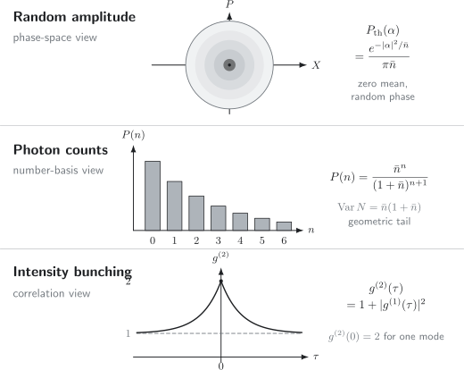
One thermal mode has a zero-centered Gaussian amplitude ensemble, a geometric photon-number distribution, and $g^{(2)}(0)=2$. A physical finite-bandwidth field loses intensity correlation outside its coherence time, so $g^{(2)}(\tau)$ returns to one.

Thermal Versus Phase-Randomized Coherent Light

A phase-randomized coherent state with mean $\bar n$ is

$$\rho_{\mathrm{PRC}} = \int_0^{2\pi} \frac{d\phi}{2\pi} \lvert \sqrt{\bar n}e^{i\phi} \rangle \langle \sqrt{\bar n}e^{i\phi} \rvert.$$

It is number diagonal, just like a thermal state, but its number distribution is Poisson:

$$P_{\mathrm{PRC}}(n) = e^{-\bar n} \frac{\bar n^n}{n!}.$$

The comparison is:

Property	Phase-randomized coherent	Thermal
$\langle a\rangle$	$0$	$0$
phase-space amplitude	fixed radius, random phase	Gaussian radius and phase
number law	Poisson	geometric
variance	$\bar n$	$\bar n(1+\bar n)$
$g^{(2)}(0)$	$1$	$2$
positive $P$ model	ring distribution	circular Gaussian

Random phase alone does not create thermal light. Thermal statistics require amplitude fluctuations with the appropriate exponential intensity law.

Photon Bunching

The normalized equal-time second-order coherence is

$$g^{(2)}(0) = \frac{ \langle \hat a^\dagger\hat a^\dagger\hat a\hat a \rangle }{ \langle\hat a^\dagger\hat a\rangle^2 } = \frac{ \langle N(N-1)\rangle }{ \bar n^2 }.$$

For one ideal thermal mode,

$$g^{(2)}(0)=2.$$

Conditioned on a detection, a second detection is twice as likely at zero delay as it is at delays much longer than the field coherence time, under the ideal stationary single-mode assumptions.

The phrase photon bunching describes this enhanced coincidence probability. It does not mean that photons exert an attractive force or travel in rigid packets. In a positive-$P$ description, the field intensity fluctuates: detections are more likely during bright fluctuations, and a first detection updates the observer toward such a bright interval.

Higher orders

For one thermal mode,

$$\left\langle (\hat a^\dagger)^m\hat a^m \right\rangle = m!\,\bar n^m.$$

Therefore

$$g^{(m)}(0)=m!.$$

Thermal fluctuations become increasingly distinct from coherent factorization at higher order. Measuring only $g^{(2)}$ does not establish the entire hierarchy.

The Siegert Relation

For a zero-mean, stationary, circular complex Gaussian field, fourth-order moments factor into products of second-order moments. This gives the Siegert relation

$$g^{(2)}(x_1,x_2) = 1+ \left| g^{(1)}(x_1,x_2) \right|^2.$$

At equal spacetime points,

$$\left| g^{(1)}(x,x) \right|=1,$$

so

$$g^{(2)}(x,x)=2.$$

At separations beyond the mutual coherence region,

$$g^{(1)}(x_1,x_2)\to0,$$

and

$$g^{(2)}(x_1,x_2)\to1.$$

The relation requires Gaussian statistics and zero coherent displacement. It need not hold for arbitrary bunched fields, non-Gaussian sources, displaced thermal states, or detector records dominated by technical artifacts.

Temporal coherence

For a stationary field with normalized spectrum $S(\omega)$,

$$g^{(1)}(\tau) = \frac{ \int d\omega\, S(\omega)e^{-i\omega\tau} }{ \int d\omega\,S(\omega) }.$$

The first-order coherence time is set by spectral width. Under the Gaussian thermal assumption,

$$g^{(2)}(\tau) = 1+ \left| g^{(1)}(\tau) \right|^2.$$

For a Lorentzian spectrum with

$$g^{(1)}(\tau) = e^{-i\omega_0\tau} e^{-\gamma\lvert\tau\rvert},$$

the intensity correlation is

$$g^{(2)}(\tau) = 1+ e^{-2\gamma\lvert\tau\rvert}.$$

The bunching feature is narrower than the first-order field-coherence envelope under this convention.

Spatial coherence

At equal times,

$$g^{(2)}(\mathbf r_1,\mathbf r_2) = 1+ \left| g^{(1)}(\mathbf r_1,\mathbf r_2) \right|^2.$$

Intensity interferometry uses this relation to infer spatial coherence even when optical phase fluctuates too rapidly for direct amplitude interferometry. For a distant incoherent source, spatial coherence contains information about the source’s angular intensity distribution.

The full interferometer geometry and source-reconstruction problem belong to Hanbury Brown–Twiss Interferometry.

What an HBT Measurement Records

An optical Hanbury Brown–Twiss arrangement splits a field and time-tags detections at two outputs. A normalized coincidence histogram estimates

$$g^{(2)}(\tau)$$

after accounting for detector efficiencies, backgrounds, timing response, dead time, and normalization windows.

Thermal bunching is seen as excess coincidences near the delay over which the field remains coherent. The beam splitter does not create the thermal correlation; it routes the incident fluctuations to two detectors so they can be compared without one detector’s dead time dominating the same-channel record.

Timing resolution

If the true bunching feature is narrower than detector jitter or the correlation bin, the measured peak is averaged down:

$$g_{\mathrm{obs}}^{(2)}(0)<2.$$

A small observed excess can therefore be consistent with single-mode thermal statistics at the source. The comparison requires convolution with the instrument response and integration over the detected optical bandwidth.

Uncorrelated background

Let a single thermal signal contribute mean rate $S$ and independent Poissonian background contribute $B$. At zero delay, the excess normalized correlation is diluted:

$$g_{\mathrm{obs}}^{(2)}(0)-1 = \left( \frac{S}{S+B} \right)^2.$$

Hence

$$g_{\mathrm{obs}}^{(2)}(0) = 1+ \left( \frac{S}{S+B} \right)^2$$

for an ideal single-mode thermal signal and ideal uncorrelated background. Background subtraction without propagated uncertainty can substantially overstate bunching.

Multimode Thermal Light

Real detectors usually collect several temporal, spectral, spatial, or polarization modes. Suppose $M$ independent thermal modes have equal mean occupation and total mean

$$\mu = \sum_{j=1}^{M}\bar n_j.$$

For equal modes,

$$\bar n_j=\frac{\mu}{M}.$$

The total-count generating function is

$$G_M(z) = \left[ 1+ \frac{\mu}{M} (1-z) \right]^{-M}.$$

The resulting negative-binomial distribution is

$$\begin{aligned} P_M(n) ={}& \binom{n+M-1}{n} \left( \frac{M}{M+\mu} \right)^M \\ &\times \left( \frac{\mu}{M+\mu} \right)^n. \end{aligned}$$

Its mean and variance are

$$\langle N\rangle=\mu,$$ $$\operatorname{Var}(N) = \mu+\frac{\mu^2}{M}.$$

Therefore

$$g^{(2)}(0) = 1+\frac1M.$$

As more independent modes are averaged,

$$g^{(2)}(0)\to1.$$

This does not turn each mode into a coherent state. It is a central-limit effect in the summed intensity.

Unequal modes and effective mode number

For independent thermal modes with means $\bar n_j$,

$$\langle N\rangle = \sum_j\bar n_j,$$

and

$$\operatorname{Var}(N) = \sum_j \bar n_j(1+\bar n_j).$$

The normalized correlation is

$$g^{(2)}(0) = 1+ \frac{ \sum_j\bar n_j^2 }{ \left( \sum_j\bar n_j \right)^2 }.$$

Define

$$M_{\mathrm{eff}} = \frac{ \left( \sum_j\bar n_j \right)^2 }{ \sum_j\bar n_j^2 }.$$

Then

$$g^{(2)}(0) = 1+ \frac1{M_{\mathrm{eff}}}.$$

The effective mode number is an inverse participation ratio. It equals the integer $M$ only for equally weighted modes.

Polarization must be counted. Detecting two uncorrelated polarization modes with equal intensity gives

$$g^{(2)}(0)=\frac32,$$

not $2$.

Pure Loss and Thermal Light

A pure-loss channel of transmissivity $\eta$ transforms the number generating function by

$$G_{\mathrm{out}}(z) = G_{\mathrm{in}} \left( 1-\eta+\eta z \right).$$

For one thermal mode,

$$G_{\mathrm{in}}(z) = \frac1{ 1+\bar n(1-z) }.$$

Therefore

$$G_{\mathrm{out}}(z) = \frac1{ 1+\eta\bar n(1-z) }.$$

The output is another thermal state with

$$\bar n_{\mathrm{out}} = \eta\bar n.$$

Ideal uniform loss preserves

$$g^{(2)}(0)=2$$

for a single resolved mode, even though brightness and signal-to-background ratio decrease. Mode-dependent loss can change the effective mode number and therefore the observed bunching.

Relation to Blackbody Radiation

In an ideal cavity at temperature $T$, each electromagnetic normal mode has

$$\bar n(\omega,T) = \frac1{ e^{\hbar\omega/(k_{\mathrm B}T)}-1 }.$$

The number of free-space modes per volume per angular-frequency interval, including two transverse polarizations, is

$$\frac{dM}{V\,d\omega} = \frac{\omega^2}{\pi^2c^3}.$$

Multiplying mode density by thermal energy per photon gives the Planck energy density

$$u(\omega,T) = \frac{ \hbar\omega^3 }{ \pi^2c^3 } \frac1{ e^{\hbar\omega/(k_{\mathrm B}T)}-1 }.$$

This expression omits the formal zero-point contribution $\hbar\omega/2$ per mode because blackbody emission and ordinary thermal energy measurements concern the temperature-dependent excitation energy.

In ordinary frequency $\nu=\omega/(2\pi)$,

$$u(\nu,T) = \frac{ 8\pi h\nu^3 }{ c^3 } \frac1{ e^{h\nu/(k_{\mathrm B}T)}-1 }.$$

Low- and high-frequency limits

When

$$\hbar\omega\ll k_{\mathrm B}T,$$

the mean occupation is

$$\bar n \approx \frac{ k_{\mathrm B}T }{ \hbar\omega }.$$

The mean mode energy approaches $k_{\mathrm B}T$, recovering the Rayleigh–Jeans limit.

When

$$\hbar\omega\gg k_{\mathrm B}T,$$

the occupation is exponentially small:

$$\bar n \approx e^{-\hbar\omega/(k_{\mathrm B}T)}.$$

Planck’s law describes the mean spectral energy density. The geometric one-mode distribution and correlation hierarchy provide additional information not visible in the mean spectrum alone.

Why blackbody bunching is hard to see optically

Broadband blackbody light has a very short coherence time. Slow detectors and wide timing bins average over many independent temporal modes, pushing the measured $g^{(2)}(0)$ toward one. Narrow spectral filtering lengthens the coherence time but discards flux.

Spatial collection likewise matters. A large detector aperture or extended source may combine many coherence areas. Observing near-ideal bunching requires resolving a small enough set of spatiotemporal and polarization modes.

Physical Sources

Equilibrium cavities and blackbodies

A cavity weakly coupled to walls at temperature $T$ approaches a product of thermal states in its independent normal modes under the ideal equilibrium model. Radiation escaping a small aperture samples that field.

Real surfaces have frequency- and angle-dependent emissivity. A graybody or selective emitter can have thermal occupation weighted by its coupling and transmission rather than unit blackbody emissivity.

Independent spontaneous emitters

Light from many independent atoms, molecules, or microscopic current sources can approach a zero-mean Gaussian field through addition of many random complex amplitudes. Gas-discharge lamps and fluorescence can exhibit chaotic statistics after suitable mode selection.

The field need not be in thermodynamic equilibrium with a single temperature. Gaussian chaotic statistics concern amplitude correlations; thermal equilibrium is the stronger thermodynamic statement.

Amplified spontaneous emission

Amplified spontaneous emission can be bright and bunched. Gain, filtering, saturation, and propagation set its spectrum and mode number. It may approximate thermal or Gaussian light in selected modes while remaining a nonequilibrium source.

Pseudo-thermal light

A coherent laser scattered from a rotating diffuser can produce a fluctuating speckle pattern. At a fixed point, the sum of many random phasors may be approximately circular Gaussian, giving

$$g^{(2)}(0)\approx2$$

and a tunable coherence time set by diffuser motion.

Such light is useful because it can provide much higher brightness and longer correlation times than a blackbody at optical frequencies. It is called pseudo-thermal because its spectrum, stationarity, higher correlations, or global mode structure need not equal an equilibrium Gibbs field.

What Thermal Light Is Not

Thermal light is not:

• a coherent state with merely unknown phase;
• proof that photons attract one another;
• necessarily broadband;
• necessarily in equilibrium whenever $g^{(2)}(0)>1$;
• nonclassical merely because it bunches;
• guaranteed to yield an observed peak of exactly two;
• described completely by Planck’s mean spectrum;
• a single mode unless the apparatus resolves one.

A Practical Analysis Workflow

When a source is called thermal:

1. Define the detected modes. Include time, bandwidth, spatial profile, and polarization.
2. Separate thermodynamics from Gaussian statistics. State whether a temperature and Gibbs state are physically justified.
3. Write the one-mode or multimode state. Use a geometric law for each independent thermal mode.
4. Compute the effective mode number. Weight modes by detected mean occupation rather than simply counting nominal channels.
5. Specify detector response. Convolve timing jitter and binning with the predicted correlation function.
6. Include background and loss. Uniform loss preserves ideal normalized correlations, but background and mode-dependent transmission do not.
7. Test the appropriate hierarchy. The Siegert relation and higher-order moments are stronger tests than one $g^{(2)}(0)$ value.
8. Report bandwidth and normalization. Coherence times and bunching amplitudes are meaningless without them.

Common Mistakes

Using a Poisson law for one thermal mode

The one-mode thermal distribution is geometric. Poisson statistics describe an ideal coherent state.

Treating mean occupation as a fixed number

The Bose–Einstein value $\bar n$ is an ensemble mean. A thermal number measurement fluctuates with variance $\bar n(1+\bar n)$.

Calling random phase sufficient

A fixed-amplitude random-phase ensemble remains Poissonian. Thermal light requires the Gaussian amplitude distribution that produces exponential intensity fluctuations.

Calling bunching uniquely quantum

Ideal thermal light has a positive $P$ representation and its bunching can be reproduced by classical random intensity plus quantum photodetection. Values below the classical bounds, not bunching itself, witness optical nonclassicality.

Expecting every measurement to give two

Multiple modes, polarization averaging, timing jitter, background, and finite bin width all reduce the observed peak.

Applying the Siegert relation to any noisy field

The relation assumes zero-mean circular Gaussian statistics. Non-Gaussian fluctuations or coherent displacement add other terms.

Ignoring the mode dependence of temperature

The same temperature produces very different $\bar n$ at microwave and optical frequencies because the relevant ratio is $\hbar\omega/(k_{\mathrm B}T)$.

Adding zero-point energy to emitted blackbody power

The Planck thermal spectrum counts excitations above vacuum. A formal vacuum energy density is not ordinary radiated thermal power.

Equating pseudo-thermal with equilibrium

An engineered source can reproduce a bunching curve without satisfying a global Gibbs state or Planck spectrum.

Inferring coherence from spectral width alone

Spectrum fixes first-order temporal coherence under stationarity. It does not by itself determine photon statistics or higher-order correlations.

Connections

• Phase-Space Distributions compares the positive thermal $P$, Wigner, and $Q$ Gaussians and their ordering-dependent widths.
• Quantum Optics supplies the state–transformation–measurement map.
• Quantized Electromagnetic Modes defines the modes to which thermal occupations are assigned.
• Photon Number States develops the number basis and factorial-moment diagnostics.
• Coherent Light provides the Poisson and displaced-vacuum comparison.
• Squeezed Light contrasts isotropic thermal Gaussian noise with an anisotropic sub-vacuum quadrature.
• Bose–Einstein Statistics is the canonical home for the equilibrium bosonic occupation law.
• Occupation Numbers separates basis states, distributions, means, and count records.
• Blackbody Radiation gives the experimental and historical route to Planck’s spectrum.
• Thermal and Vacuum Noise treats bath correlations, detailed balance, and oscillator relaxation.
• Photon Counting owns detector records, efficiency, dark counts, and continuous monitoring.
• Gaussian States and Wigner Functions gives the broader continuous-variable Gaussian-state framework.

Exercises

1. Normalize the one-mode thermal state

Starting from

$$\rho = C \sum_{n=0}^{\infty} q^n \lvert n\rangle\langle n\rvert, \qquad 0\le q<1,$$

find $C$, $\bar n$, and $q$ in terms of $\bar n$.

Solution

Normalization requires

$$1 = C \sum_{n=0}^{\infty}q^n = \frac{C}{1-q}.$$

Therefore

$$C=1-q.$$

The mean is

$$\bar n = (1-q) \sum_{n=0}^{\infty} nq^n.$$

Using

$$\sum_{n=0}^{\infty} nq^n = \frac{q}{(1-q)^2},$$

one gets

$$\bar n = \frac{q}{1-q}.$$

Solving,

$$q = \frac{\bar n}{1+\bar n}.$$

Hence

$$\rho = \frac1{1+\bar n} \sum_{n=0}^{\infty} \left( \frac{\bar n}{1+\bar n} \right)^n \lvert n\rangle\langle n\rvert.$$

2. Thermal factorial moments

Use the generating function to show

$$\langle N(N-1)\rangle=2\bar n^2$$

and derive $g^{(2)}(0)$ and $\operatorname{Var}(N)$.

Solution

The generating function is

$$G(z) = \frac{1-q}{1-qz}.$$

Its derivatives are

$$G'(z) = \frac{ (1-q)q }{ (1-qz)^2 },$$

and

$$G''(z) = \frac{ 2(1-q)q^2 }{ (1-qz)^3 }.$$

At $z=1$,

$$\langle N\rangle = \frac{q}{1-q} = \bar n,$$

and

$$\langle N(N-1)\rangle = \frac{2q^2}{(1-q)^2} = 2\bar n^2.$$

Therefore

$$g^{(2)}(0) = \frac{2\bar n^2}{\bar n^2} = 2.$$

Finally,

$$\begin{aligned} \operatorname{Var}(N) &= \langle N(N-1)\rangle + \langle N\rangle - \langle N\rangle^2 \\ &= \bar n(1+\bar n). \end{aligned}$$

3. Thermal quadratures and purity

Show that

$$(\Delta X)^2 = (\Delta P)^2 = \bar n+\frac12$$

and verify

$$\operatorname{Tr}(\rho_{\mathrm{th}}^2) = \frac1{2\bar n+1}.$$

Solution

Because the state is number diagonal,

$$\langle a\rangle = \langle a^2\rangle = 0.$$

Also,

$$\langle a^\dagger a\rangle=\bar n, \qquad \langle aa^\dagger\rangle=\bar n+1.$$

Thus

$$\begin{aligned} \langle X^2\rangle &= \frac12 \left\langle a^2+aa^\dagger+a^\dagger a+(a^\dagger)^2 \right\rangle \\ &= \bar n+\frac12. \end{aligned}$$

Since $\langle X\rangle=0$, this is the variance. The same calculation gives the $P$ variance.

For purity,

$$\begin{aligned} \operatorname{Tr}(\rho^2) &= (1-q)^2 \sum_{n=0}^{\infty}q^{2n} \\ &= \frac{(1-q)^2}{1-q^2} \\ &= \frac{1-q}{1+q}. \end{aligned}$$

Using $q=\bar n/(1+\bar n)$ gives

$$\operatorname{Tr}(\rho^2) = \frac1{2\bar n+1}.$$

4. Thermal light through loss

Use Bernoulli thinning to show that a thermal input with mean $\bar n$ remains thermal after pure loss of transmissivity $\eta$. Find the output mean and $g^{(2)}(0)$.

Solution

For an input generating function $G_{\mathrm{in}}(z)$, independent survival with probability $\eta$ replaces

$$z \longmapsto 1-\eta+\eta z.$$

The thermal generating function is

$$G_{\mathrm{in}}(z) = \frac1{ 1+\bar n(1-z) }.$$

Hence

$$\begin{aligned} G_{\mathrm{out}}(z) &= \frac1{ 1+\bar n \left[ 1-(1-\eta+\eta z) \right] } \\ &= \frac1{ 1+\eta\bar n(1-z) }. \end{aligned}$$

This is thermal with

$$\bar n_{\mathrm{out}} = \eta\bar n.$$

Its factorial second moment is

$$\langle N_{\mathrm{out}} (N_{\mathrm{out}}-1)\rangle = 2(\eta\bar n)^2.$$

Therefore

$$g_{\mathrm{out}}^{(2)}(0)=2.$$

Uniform loss changes brightness but not the normalized ideal single-mode bunching.

5. Equal multimode thermal counts

For $M$ independent equal thermal modes with total mean $\mu$, derive the variance and $g^{(2)}(0)$ of the total count.

Solution

Each mode has mean

$$\bar n_j=\frac{\mu}{M}$$

and variance

$$\operatorname{Var}(N_j) = \frac{\mu}{M} \left( \frac{\mu}{M} \right)^2.$$

Independence makes variances add:

$$\begin{aligned} \operatorname{Var}(N) &= M \left[ \frac{\mu}{M} + \frac{\mu^2}{M^2} \right] \\ &= \mu+\frac{\mu^2}{M}. \end{aligned}$$

Using

$$g^{(2)}(0) = 1+ \frac{ \operatorname{Var}(N)-\mu }{ \mu^2 },$$

one obtains

$$g^{(2)}(0) = 1+\frac1M.$$

For $M=1$ the value is $2$; for many modes it approaches one.

6. Unequal effective mode number

Three independent thermal modes have detected means $4$, $2$, and $1$. Compute $M_{\mathrm{eff}}$ and $g^{(2)}(0)$.

Solution

The total mean is

$$\sum_j\bar n_j = 4+2+1 = 7.$$

The squared-weight sum is

$$\sum_j\bar n_j^2 = 16+4+1 = 21.$$

Therefore

$$M_{\mathrm{eff}} = \frac{7^2}{21} = \frac73.$$

The normalized correlation is

$$\begin{aligned} g^{(2)}(0) &= 1+\frac1{M_{\mathrm{eff}}} \\ &= 1+\frac37 \\ &= \frac{10}{7}. \end{aligned}$$

The effective mode number is not an integer because the three modes are unequally weighted.

7. Coherence and bunching widths

A zero-mean Gaussian field has

$$g^{(1)}(\tau) = e^{-i\omega_0\tau} e^{-\gamma\lvert\tau\rvert}.$$

Find $g^{(2)}(\tau)$ and the half-maximum delay of its excess above one.

Solution

The Siegert relation gives

$$\begin{aligned} g^{(2)}(\tau) &= 1+ \left| g^{(1)}(\tau) \right|^2 \\ &= 1+ e^{-2\gamma\lvert\tau\rvert}. \end{aligned}$$

The excess above baseline is

$$g^{(2)}(\tau)-1 = e^{-2\gamma\lvert\tau\rvert}.$$

At half maximum,

$$e^{-2\gamma\lvert\tau_{1/2}\rvert} = \frac12.$$

Thus

$$\lvert\tau_{1/2}\rvert = \frac{\ln2}{2\gamma}.$$

The full width at half maximum of the bunching excess is

$$\frac{\ln2}{\gamma}.$$

8. Random phase is not thermal

At mean photon number $\bar n=1$, compare one thermal mode with a phase-randomized coherent state. Compute $P(0)$, $P(1)$, and $g^{(2)}(0)$ for each.

Solution

For the thermal state,

$$P_{\mathrm{th}}(n) = \frac1{1+\bar n} \left( \frac{\bar n}{1+\bar n} \right)^n.$$

At $\bar n=1$,

$$P_{\mathrm{th}}(0)=\frac12, \qquad P_{\mathrm{th}}(1)=\frac14,$$

and

$$g_{\mathrm{th}}^{(2)}(0)=2.$$

The phase-randomized coherent state has the Poisson law

$$P_{\mathrm{PRC}}(n) = e^{-1}\frac1{n!}.$$

Thus

$$P_{\mathrm{PRC}}(0)=e^{-1}, \qquad P_{\mathrm{PRC}}(1)=e^{-1},$$

and

$$g_{\mathrm{PRC}}^{(2)}(0)=1.$$

Both states have zero mean amplitude after phase averaging, but their amplitude-radius and number fluctuations are different.

References

• M. Planck, “Ueber das Gesetz der Energieverteilung im Normalspectrum,” Annalen der Physik 309, 553–563 (1901), doi:10.1002/andp.19013090310.
• R. Hanbury Brown and R. Q. Twiss, “Correlation between Photons in Two Coherent Beams of Light,” Nature 177, 27–29 (1956), doi:10.1038/177027a0.
• R. Hanbury Brown and R. Q. Twiss, “A Test of a New Type of Stellar Interferometer on Sirius,” Nature 178, 1046–1048 (1956), doi:10.1038/1781046a0.
• R. J. Glauber, “The Quantum Theory of Optical Coherence,” Physical Review 130, 2529–2539 (1963), doi:10.1103/PhysRev.130.2529.
• R. J. Glauber, “Coherent and Incoherent States of the Radiation Field,” Physical Review 131, 2766–2788 (1963), doi:10.1103/PhysRev.131.2766.
• F. T. Arecchi, E. Gatti, and A. Sona, “Time Distribution of Photons from Coherent and Gaussian Sources,” Physics Letters 20, 27–29 (1966), doi:10.1016/0031-9163(66)91034-1.
• L. Mandel and E. Wolf, Optical Coherence and Quantum Optics, Cambridge University Press (1995), doi:10.1017/CBO9781139644105.
• R. Loudon, The Quantum Theory of Light, 3rd ed., Oxford University Press (2000).
• M. O. Scully and M. S. Zubairy, Quantum Optics, Cambridge University Press (1997), doi:10.1017/CBO9780511813993.
• G. Grynberg, A. Aspect, and C. Fabre, Introduction to Quantum Optics: From the Semi-Classical Approach to Quantized Light, Cambridge University Press (2010), doi:10.1017/CBO9780511778261.
• J. Zmuidzinas, “Thermal Noise and Correlations in Photon Detection,” Applied Optics 42, 4989–5008 (2003), doi:10.1364/AO.42.004989.
• D. F. Walls and G. J. Milburn, Quantum Optics, 2nd ed., Springer (2008), doi:10.1007/978-3-540-28574-8.