Coherent Light

Coherent light is the electromagnetic realization of a bosonic coherent state. For one declared optical mode,

$$\hat a\lvert\alpha\rangle = \alpha\lvert\alpha\rangle, \qquad \alpha\in\mathbb C.$$

The complex amplitude $\alpha$ fixes the mean field relative to a phase reference, while

$$\bar n = \langle\hat a^\dagger\hat a\rangle = \lvert\alpha\rvert^2$$

is the mean photon number in that mode. The state has Poisson number statistics, vacuum-level noise in every quadrature, and factorized normally ordered correlation functions. These properties make it the quantum state closest to an ideal deterministic classical wave.

“Coherent” has several meanings in optics. They must not be silently identified:

• a coherent state is a specific quantum state $\lvert\alpha\rangle$;
• first-order coherence describes field-amplitude correlations and fringe visibility;
• higher-order coherence describes factorization of photodetection correlations;
• a laser is a driven, dissipative source whose output can approximate coherent light over specified modes and times.

A field may have excellent first-order coherence without being in a pure coherent state. Conversely, an ideal coherent pulse can be broadband. Spectral narrowness, phase stability, Poisson statistics, and coherent-state purity are related operational properties, not synonyms.

Canonical Scope

The oscillator identity

$$\lvert\alpha\rangle = \hat D(\alpha)\lvert0\rangle$$

and its number-basis derivation are canonical on Coherent States. The Wigner function and phase-plane geometry are canonical on Coherent States in Phase Space.

This page owns the optical interpretation:

• the relation between $\alpha$ and a classical electromagnetic field;
• photon counting and all-order optical correlations;
• multimode coherent pulses and mode matching;
• stability under passive linear optics and pure loss;
• phase references and phase-averaged laser descriptions;
• the conditions under which real laser output is well approximated by coherent light.

The phrase “one laser mode” always denotes an approximation. A propagating beam has spatial, polarization, frequency, and temporal structure, and a continuous-wave output occupies a sequence or continuum of temporal modes.

One-Mode Definition

For a normalized mode $f$, let

$$[\hat a_f,\hat a_f^\dagger]=1.$$

Its coherent state satisfies

$$\hat a_f\lvert\alpha_f\rangle = \alpha_f\lvert\alpha_f\rangle.$$

Equivalently,

$$\lvert\alpha_f\rangle = \hat D_f(\alpha_f)\lvert0_f\rangle,$$

where

$$\hat D_f(\alpha) = \exp\left( \alpha\hat a_f^\dagger - \alpha^*\hat a_f \right).$$

The displacement operator translates the vacuum in phase space without changing its covariance matrix.

Number-basis content

The coherent state expands as

$$\lvert\alpha\rangle = e^{-\lvert\alpha\rvert^2/2} \sum_{n=0}^{\infty} \frac{\alpha^n}{\sqrt{n!}} \lvert n\rangle.$$

It is therefore not a state of definite photon number unless $\alpha=0$, in which case it is the vacuum. The phase of $\alpha$ appears in the relative phases between neighboring number amplitudes:

$$\alpha = \sqrt{\bar n}\,e^{i\phi}.$$

Changing $\phi$ rotates the state in optical phase space.

The overlap of two coherent states is

$$\langle\beta\vert\alpha\rangle = \exp\left[ -\frac12\lvert\beta\rvert^2 -\frac12\lvert\alpha\rvert^2 +\beta^*\alpha \right].$$

Thus

$$\lvert\langle\beta\vert\alpha\rangle\rvert^2 = e^{-\lvert\alpha-\beta\rvert^2}.$$

Distinct amplitudes are never exactly orthogonal at finite separation. This fact matters in optical communication, state discrimination, and the interpretation of a “classical amplitude alphabet.”

Coherent States of Electromagnetic Modes

For a collection of orthonormal radiation modes labeled by $\mu$, a multimode coherent state is the simultaneous annihilation-operator eigenstate

$$\hat a_\mu \lvert\{\alpha\}\rangle = \alpha_\mu \lvert\{\alpha\}\rangle$$

for every $\mu$. It factorizes in that mode basis:

$$\lvert\{\alpha\}\rangle = \bigotimes_\mu \lvert\alpha_\mu\rangle.$$

Equivalently,

$$\lvert\{\alpha\}\rangle = \hat D[\alpha]\lvert0\rangle,$$

with

$$\hat D[\alpha] = \exp\left[ \sum_\mu \left( \alpha_\mu\hat a_\mu^\dagger - \alpha_\mu^*\hat a_\mu \right) \right].$$

The mean total photon number is

$$\bar N = \sum_\mu\lvert\alpha_\mu\rvert^2.$$

For continuum-normalized modes, the sum becomes an integral and the amplitude must be square integrable for a finite-energy pulse.

Coherent wave-packet modes

Suppose a normalized packet mode is

$$\hat a_f = \sum_\mu f_\mu^*\hat a_\mu, \qquad \sum_\mu\lvert f_\mu\rvert^2=1.$$

A coherent state occupying only this packet mode has amplitudes

$$\alpha_\mu = \alpha f_\mu.$$

Its total mean photon number is

$$\sum_\mu \lvert\alpha f_\mu\rvert^2 = \lvert\alpha\rvert^2.$$

The packet envelope $f_\mu$ determines where and when the pulse couples to an apparatus; $\alpha$ determines its overall complex amplitude.

If an experiment selects a different normalized mode $g$, the measured coherent amplitude is the overlap projection

$$\alpha_g = \langle g\vert f\rangle\alpha.$$

Orthogonal components appear as loss to that measurement. This is why local oscillator mode matching is part of a homodyne measurement, not a cosmetic alignment detail.

Mean Electromagnetic Field

Write the positive-frequency electric-field operator as

$$\hat{\mathbf E}^{(+)}(x) = \sum_\mu \boldsymbol{\mathcal E}_\mu(x) \hat a_\mu,$$

where $x=(\mathbf r,t)$ and the mode functions include the chosen normalization and free time dependence. In a multimode coherent state,

$$\langle \hat{\mathbf E}^{(+)}(x) \rangle = \sum_\mu \boldsymbol{\mathcal E}_\mu(x) \alpha_\mu.$$

Define

$$\mathbf E_{\mathrm{cl}}^{(+)}(x) \equiv \sum_\mu \boldsymbol{\mathcal E}_\mu(x) \alpha_\mu.$$

Then

$$\langle\hat{\mathbf E}(x)\rangle = \mathbf E_{\mathrm{cl}}^{(+)}(x) + \mathbf E_{\mathrm{cl}}^{(-)}(x).$$

Because expectation values respect the linear source-free Maxwell equations, this mean field evolves as a classical electromagnetic solution in a linear lossless medium. The quantum state also contains fluctuations that the mean field alone does not describe.

Single-mode amplitude

For a one-mode field written schematically as

$$\hat E^{(+)}(t) = \mathcal E_0 \hat a e^{-i\omega t},$$

one has

$$\langle\hat E(t)\rangle = 2\mathcal E_0 \lvert\alpha\rvert \cos\left( \omega t-\phi+\phi_0 \right),$$

where $\phi=\arg\alpha$ and $\phi_0$ depends on the mode convention. Changing an $i$ factor in the field expansion shifts $\phi_0$ but changes no observable prediction.

The vacuum field scale $\mathcal E_0$ is fixed by mode normalization. Thus equal numerical values of $\alpha$ in two differently confined modes need not correspond to equal electric-field amplitudes.

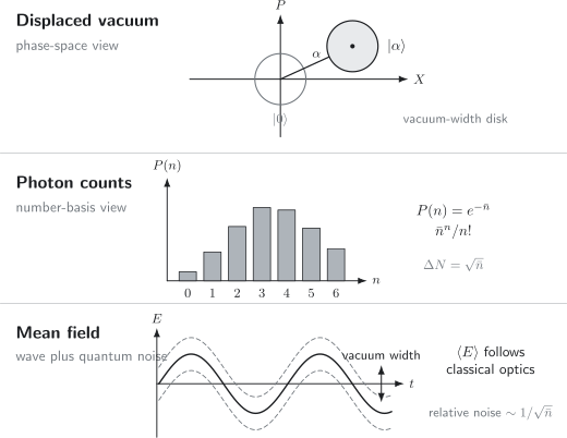
A coherent state is one structure seen three ways. It is a displaced vacuum-width Gaussian in phase space, has a Poisson photon-number distribution, and carries a classical mean field while retaining irreducible quadrature noise.

Photon Number Statistics

Taking the modulus squared of the number-basis coefficients gives

$$P(n) = e^{-\bar n} \frac{\bar n^n}{n!}, \qquad \bar n=\lvert\alpha\rvert^2.$$

This is a Poisson distribution. Its mean and variance are

$$\langle\hat N\rangle=\bar n, \qquad (\Delta N)^2=\bar n.$$

Therefore

$$F = \frac{(\Delta N)^2}{\langle\hat N\rangle} = 1,$$

and the Mandel parameter is

$$Q=F-1=0.$$

Poisson statistics lie between sub-Poissonian number squeezing and super-Poissonian excess noise. They do not mean “no noise.” The standard deviation is

$$\Delta N=\sqrt{\bar n}.$$

Only the relative number noise decreases:

$$\frac{\Delta N}{\bar n} = \frac{1}{\sqrt{\bar n}}.$$

Factorial moments

Because $\lvert\alpha\rangle$ is an annihilation-operator eigenstate,

$$\left\langle (\hat a^\dagger)^m\hat a^m \right\rangle = \lvert\alpha\rvert^{2m} = \bar n^m.$$

Equivalently,

$$\left\langle \hat N(\hat N-1)\cdots(\hat N-m+1) \right\rangle = \bar n^m.$$

Every normalized equal-mode correlation is therefore

$$g^{(m)}(0)=1$$

where the normalization is defined and $\bar n>0$. In particular,

$$g^{(2)}(0)=1.$$

This is neither bunching nor antibunching. It is the correlation value of a Poisson process in the ideal single-mode model.

Count distribution

For ideal direct detection of a coherent mode during a gate that contains mean photon number $\bar n$, the count distribution is Poisson:

$$P(K=k) = e^{-\bar n} \frac{\bar n^k}{k!}.$$

Independent detection efficiency $\eta$ thins a Poisson process into another Poisson process:

$$P_\eta(K=k) = e^{-\eta\bar n} \frac{ (\eta\bar n)^k }{ k! }.$$

For an ideal on–off detector,

$$P(\text{no click}) = e^{-\eta\bar n},$$ $$P(\text{click}) = 1-e^{-\eta\bar n}.$$

Background counts, technical intensity noise, dead time, saturation, and multimode fluctuations can all spoil this simple law.

Optical Correlation Functions

Glauber photodetection theory uses normally ordered correlation functions. For $m$ detections,

$$\begin{aligned} & G^{(m)} \left( x_1,\ldots,x_m; y_m,\ldots,y_1 \right) \\ &= \left\langle \begin{gathered} \hat E^{(-)}(x_1)\cdots \hat E^{(-)}(x_m) \\ {}\times \hat E^{(+)}(y_m)\cdots \hat E^{(+)}(y_1) \end{gathered} \right\rangle. \end{aligned}$$

For a coherent state, each positive-frequency field operator acts by its classical eigenvalue. Therefore

$$\begin{aligned} G^{(m)} ={}& \prod_{j=1}^{m} E_{\mathrm{cl}}^{(-)}(x_j) \\ &\times \prod_{j=1}^{m} E_{\mathrm{cl}}^{(+)}(y_j). \end{aligned}$$

All normally ordered correlations factorize. This is the precise sense in which an ideal coherent state is fully coherent in Glauber’s hierarchy.

First-order coherence

The first-order function is

$$G^{(1)}(x,y) = \left\langle \hat E^{(-)}(x) \hat E^{(+)}(y) \right\rangle.$$

For coherent light,

$$G^{(1)}(x,y) = E_{\mathrm{cl}}^{(-)}(x) E_{\mathrm{cl}}^{(+)}(y).$$

This rank-one factorization gives ideal fringe visibility when the two sampled fields have matched polarization and intensity.

First-order coherence alone does not identify a coherent state. For example, a stationary one-mode number state can have perfect normalized first-order coherence while exhibiting

$$g^{(2)}(0)=1-\frac1n.$$

The hierarchy matters.

Second-order coherence

For one stationary mode,

$$g^{(2)}(\tau) = \frac{ \left\langle \hat a^\dagger(t) \hat a^\dagger(t+\tau) \hat a(t+\tau) \hat a(t) \right\rangle }{ \langle\hat N(t)\rangle \langle\hat N(t+\tau)\rangle }.$$

An ideal coherent state under linear harmonic evolution gives

$$g^{(2)}(\tau)=1$$

for every delay. A measured value near one is consistent with coherent light, but it is not sufficient evidence: many noncoherent states and noisy mixtures can share the same second-order value.

Minimum-Uncertainty Quadratures

Adopt the dimensionless quadratures

$$\hat X = \frac{ \hat a+\hat a^\dagger }{ \sqrt2 }, \qquad \hat P = \frac{ \hat a-\hat a^\dagger }{ i\sqrt2 }.$$

They satisfy

$$[\hat X,\hat P]=i.$$

In $\lvert\alpha\rangle$,

$$\langle\hat X\rangle = \sqrt2\,\operatorname{Re}\alpha,$$ $$\langle\hat P\rangle = \sqrt2\,\operatorname{Im}\alpha.$$

The variances are

$$(\Delta X)^2 = (\Delta P)^2 = \frac12,$$

so

$$\Delta X\,\Delta P = \frac12.$$

These are the vacuum variances in this convention. Some texts define quadratures with an extra factor of $\sqrt2$ or $2$, changing every displayed variance. A quoted “shot-noise unit” is incomplete without the normalization.

Rotated quadrature

The phase-referenced quadrature

$$\hat X_\theta = \frac{ \hat a e^{-i\theta} + \hat a^\dagger e^{i\theta} }{ \sqrt2 }$$

has mean

$$\langle\hat X_\theta\rangle = \sqrt2\, \operatorname{Re} \left( \alpha e^{-i\theta} \right),$$

and variance

$$(\Delta X_\theta)^2 = \frac12$$

for every $\theta$. The uncertainty disk is translated but not squeezed.

At the optimal phase, $\theta=\arg\alpha$, the mean-to-noise ratio is

$$\frac{ \lvert\langle X_\theta\rangle\rvert }{ \Delta X_\theta } = 2\lvert\alpha\rvert = 2\sqrt{\bar n}.$$

The absolute quadrature noise remains fixed while the signal grows.

Wigner function

With complex phase-space coordinate $\beta$, the one-mode Wigner function is

$$W_\alpha(\beta) = \frac{2}{\pi} \exp\left[ -2\lvert\beta-\alpha\rvert^2 \right].$$

It is a positive Gaussian centered at $\alpha$ with the same width as the vacuum. Positivity here is consistent with the coherent state lying at the classical boundary of the Glauber–Sudarshan description. The state remains fully quantum: it has irreducible noise, nonorthogonal alternatives, and measurement backaction.

Phase and the Reference Problem

Write

$$\alpha = \sqrt{\bar n}\,e^{i\phi}.$$

The angle $\phi$ determines the mean field relative to a clock or local oscillator. Under an optical phase shift,

$$\hat U(\vartheta) = e^{-i\vartheta\hat N},$$

the state transforms as

$$\hat U(\vartheta) \lvert\alpha\rangle = \lvert \alpha e^{-i\vartheta} \rangle.$$

Absolute phase is not read without a reference. Interference, homodyne, and heterodyne measurements compare the signal with another path or mode whose phase defines the coordinate system.

Unknown phase is a mixed-state description

If the phase is uniformly unknown relative to the available reference frame, the appropriate phase-averaged state is

$$\rho_{\mathrm{av}} = \int_0^{2\pi} \frac{d\phi}{2\pi} \lvert \sqrt{\bar n}e^{i\phi} \rangle \langle \sqrt{\bar n}e^{i\phi} \rvert.$$

Expanding in number states gives

$$\rho_{\mathrm{av}} = e^{-\bar n} \sum_{n=0}^{\infty} \frac{\bar n^n}{n!} \lvert n\rangle\langle n\rvert.$$

All off-diagonal number coherences vanish, and

$$\operatorname{Tr} \left( \rho_{\mathrm{av}}\hat a \right) = 0.$$

Nevertheless,

$$\left\langle (\hat a^\dagger)^m\hat a^m \right\rangle_{\mathrm{av}} = \bar n^m.$$

Direct photon counting cannot distinguish this state from a pure coherent state of known amplitude and phase because both have the same Poisson number distribution. A phase-sensitive comparison with an external reference can.

Shared unknown phase is not independent random phase

Suppose several temporal packets are drawn from one phase-stable laser during a time shorter than its coherence time. A useful joint model is

$$\rho_{\mathrm{shared}} = \int_0^{2\pi} \frac{d\phi}{2\pi} \bigotimes_j \lvert \alpha_j e^{i\phi} \rangle \langle \alpha_j e^{i\phi} \rvert.$$

All packets share the same unknown phase. This state is not

$$\bigotimes_j \left[ \int_0^{2\pi} \frac{d\phi_j}{2\pi} \lvert \alpha_j e^{i\phi_j} \rangle \langle \alpha_j e^{i\phi_j} \rvert \right],$$

which assigns independent random phases to every packet. The first model retains relative phase coherence and predicts interference between packets; the second generally does not.

This distinction resolves many apparently contradictory claims about whether a free-running laser “really” emits a coherent state. The density operator depends on the chosen subsystem, reference frame, conditioning information, and time interval. Operational predictions, not a preferred ensemble decomposition, are decisive.

Passive Linear Optics

Let a passive interferometer transform annihilation operators as

$$\hat b_j = \sum_k U_{jk}\hat a_k, \qquad U^\dagger U=I.$$

A product coherent input remains a product coherent output:

$$\bigotimes_k \lvert\alpha_k\rangle \longmapsto \bigotimes_j \lvert\beta_j\rangle,$$

where

$$\beta_j = \sum_k U_{jk}\alpha_k.$$

Thus passive linear optics acts on coherent amplitudes exactly as classical wave optics acts on complex field amplitudes.

Beam splitter

For one common beam-splitter convention,

$$\begin{aligned} \hat c &= t\hat a+r\hat b, \\ \hat d &= -r^*\hat a+t^*\hat b, \end{aligned}$$

with

$$\lvert t\rvert^2+\lvert r\rvert^2=1.$$

Then

$$\lvert\alpha\rangle_a \lvert\beta\rangle_b \longmapsto \lvert t\alpha+r\beta \rangle_c \lvert -r^*\alpha+t^*\beta \rangle_d.$$

No entanglement is generated between the outputs from product coherent inputs. This exceptional property is one reason coherent states are treated as classical optical inputs.

Pure loss

Model attenuation as a beam splitter coupling the signal to an environmental vacuum mode:

$$\lvert\alpha\rangle_S\lvert0\rangle_E \longmapsto \lvert\sqrt\eta\,\alpha\rangle_S \lvert\sqrt{1-\eta}\,\alpha\rangle_E.$$

After tracing out the environment,

$$\rho_S' = \lvert\sqrt\eta\,\alpha\rangle \langle\sqrt\eta\,\alpha\rvert.$$

An ideal coherent state remains pure and coherent under vacuum loss. Its mean photon number changes from $\bar n$ to $\eta\bar n$, while its quadrature variance remains the vacuum value.

This stability is not generic. Number states become mixtures under loss, squeezed states lose squeezing, and phase-insensitive amplification must add noise.

Coherent Driving

A classical current or strong external drive couples linearly to a bosonic mode. In a rotating frame, a common driven damped-mode equation is

$$\frac{d\alpha}{dt} = -\left( \frac{\kappa}{2}+i\Delta \right)\alpha + \varepsilon(t),$$

where $\kappa$ is the energy-decay rate, $\Delta$ the detuning, and $\varepsilon$ the drive amplitude in the chosen convention.

For constant drive,

$$\alpha_{\mathrm{ss}} = \frac{ \varepsilon }{ \kappa/2+i\Delta }.$$

A linear oscillator driven coherently and coupled to a vacuum Markovian bath relaxes toward a coherent state. Its amplitude obeys the classical response equation while the quantum covariance remains at the vacuum level.

Nonlinearity changes this conclusion. Kerr interactions, saturation, parametric processes, and strong coupling can shear, squeeze, antibunch, or entangle the field. A nonzero mean amplitude does not guarantee a coherent state.

Classical-Field Limit

Coherent states make the classical limit transparent because their mean field is a classical solution and their relative fluctuations shrink with occupation.

For photon number,

$$\frac{\Delta N}{\langle N\rangle} = \frac1{\sqrt{\bar n}}.$$

For an optimally phased quadrature,

$$\frac{ \Delta X_\phi }{ \lvert\langle X_\phi\rangle\rvert } = \frac1{2\sqrt{\bar n}}.$$

Therefore a large-amplitude coherent field supports deterministic classical predictions for coarse relative observables.

Fixed classical field as Planck’s constant changes

The single-photon electric-field scale behaves schematically as

$$\mathcal E_0 \propto \sqrt{\hbar\omega}.$$

To hold a macroscopic classical field amplitude fixed while taking $\hbar\to0$, the coherent amplitude must scale as

$$\lvert\alpha\rvert \propto \hbar^{-1/2}.$$

Then

$$\bar n=\lvert\alpha\rvert^2 \propto \hbar^{-1}.$$

The classical limit is therefore a correlated scaling, not the statement that a fixed low-occupation state becomes classical merely by naming its mean field.

What remains quantum

Even at large $\bar n$:

• the quadrature variance does not vanish in absolute oscillator units;
• coherent states with nearby amplitudes are nonorthogonal;
• shot noise remains in finite measurements;
• phase and amplitude are estimated relative to physical references;
• nonlinear interactions can convert small fluctuations into visible nonclassical effects.

Classical electromagnetism emerges for selected observables and accuracy requirements. The underlying state does not stop obeying quantum mechanics.

Coherent States and Optical Classicality

The Glauber–Sudarshan representation writes a state as

$$\rho = \int d^2\alpha\, P(\alpha) \lvert\alpha\rangle\langle\alpha\rvert.$$

A coherent state has

$$P(\beta) = \delta^{(2)}(\beta-\alpha).$$

It is therefore an extremal point of the set of states with a nonnegative classical $P$ distribution. Statistical mixtures with positive $P$ represent classical random amplitudes followed by quantum-limited photodetection.

This criterion is operationally powerful but representation specific. “Classical” here does not mean that the density operator can be replaced by a point in classical phase space for every purpose. It means its normally ordered moments admit a positive stochastic-amplitude model.

Is Laser Light a Coherent State?

An ideal coherent state is a foundational model for laser-like light, but a real laser is an open, pumped, nonlinear device with spontaneous emission, gain saturation, output coupling, technical noise, and finite bandwidth. Whether its output is accurately described by $\lvert\alpha\rangle$ depends on the subsystem and timescale.

Above-threshold amplitude

Well above threshold, gain saturation can stabilize the intracavity amplitude. A semiclassical description then has approximately fixed $\lvert\alpha\rvert$ and an oscillating field. Quantum noise continuously perturbs both amplitude and phase.

Amplitude fluctuations are often damped back toward the steady value. Phase has no corresponding restoring force in a free-running laser with continuous phase symmetry, so it diffuses. The resulting finite coherence time produces a finite laser linewidth.

Phase diffusion and linewidth

A free-running laser’s phase can diffuse even when gain saturation keeps its amplitude close to a steady value. That makes a coherent-state description conditional on mode, reference, and timescale. Linewidth and Coherence is the canonical treatment of the stochastic phase equation, first-order coherence, Lorentzian Fourier pair, Schawlow–Townes scale, technical frequency noise, and linewidth measurement.

The conclusion needed here is qualitative: over delays short compared with the phase-diffusion time, phase-conditioned coherent wave packets can be an excellent model; over long unreferenced records, averaging over the diffusing phase becomes appropriate.

Short-time coherent description

Over an interval much shorter than the phase-diffusion time, and conditioned on an estimated phase, the output can be modeled accurately as a sequence of coherent temporal modes with nearly common phase. Over much longer intervals without an external reference, phase averaging becomes appropriate.

These are not competing realities. They are descriptions conditioned on different information:

• phase tracked relative to a reference: coherent amplitudes are useful;
• phase untracked but shared across nearby packets: a common-phase mixture is useful;
• long-time single-mode reduced state: a phase-averaged Poisson mixture may be useful.

Continuous-wave output is multimode

A continuous beam cannot be assigned one finite-energy amplitude $\alpha$ for all time. One may instead use:

• finite temporal wave-packet modes;
• a photon flux with units of inverse time;
• input–output field operators satisfying delta-function commutators;
• correlation functions over detector times.

If a time bin of duration $T$ captures flux $\Phi$ in a matched mode, then schematically

$$\bar n_T \approx \Phi T,$$

provided $T$ and the mode definition are stated. Changing the bin changes $\bar n_T$ without changing the physical flux.

Real deviations

Real laser output may differ from an ideal coherent state through:

• excess intensity noise, especially near threshold or at low Fourier frequencies;
• phase diffusion and technical frequency noise;
• relaxation oscillations;
• multimode competition;
• polarization fluctuations;
• amplified spontaneous emission;
• non-Gaussian noise or intermittent mode hops;
• imperfect spatial mode quality;
• correlations introduced by stabilization loops and measurement.

Saying “laser light is coherent” is therefore a controlled approximation, not an exact universal theorem.

How to Test the Approximation

No single measurement certifies a coherent state. A useful characterization combines:

Property	Representative measurement
mean field and phase	interference or homodyne detection
first-order coherence	delayed interferometry or spectrum
photon statistics	number-resolved counting or calibrated click data
second-order coherence	Hanbury Brown–Twiss measurement
quadrature covariance	balanced homodyne detection
modal structure	spatial, spectral, and temporal mode analysis
higher-order structure	higher correlations or state tomography

Evidence consistent with an ideal coherent state includes:

$$g^{(m)}\approx1$$

over the tested orders and delays,

$$Q\approx0,$$

vacuum-level quadrature variance in every phase, and a stable displacement after accounting for phase diffusion.

Each statement is bandwidth and mode dependent. Detector dark noise can mask sub-Poissonian statistics; classical technical noise can produce super-Poissonian counts; a narrow electronic analysis band can miss noise elsewhere.

Worked Example: Coherent Light Through Loss

Start with

$$\lvert\alpha\rangle_S\lvert0\rangle_E.$$

A pure-loss channel of transmissivity $\eta$ acts as

$$\hat a_S^\dagger \longmapsto \sqrt\eta\,\hat a_S^\dagger + \sqrt{1-\eta}\,\hat a_E^\dagger.$$

Using the displacement representation,

$$\begin{aligned} \hat D_S(\alpha) &\longmapsto \hat D_S(\sqrt\eta\,\alpha) \\ &\quad\times \hat D_E(\sqrt{1-\eta}\,\alpha). \end{aligned}$$

Therefore

$$\lvert\alpha\rangle_S\lvert0\rangle_E \longmapsto \lvert\sqrt\eta\,\alpha\rangle_S \lvert\sqrt{1-\eta}\,\alpha\rangle_E.$$

The retained state has

$$\bar n_{\mathrm{out}} = \eta\lvert\alpha\rvert^2,$$ $$(\Delta N_{\mathrm{out}})^2 = \eta\lvert\alpha\rvert^2,$$

and

$$g_{\mathrm{out}}^{(2)}(0)=1.$$

The environment has learned no stochastic “which photon” record that entangles it with a coherent input; both outputs are coherent states. This factorization is special to coherent inputs.

Worked Example: A Dark Interferometer Port

Send coherent states into a balanced beam splitter with convention

$$\hat c = \frac{ \hat a+\hat b }{ \sqrt2 }, \qquad \hat d = \frac{ \hat a-\hat b }{ \sqrt2 }.$$

If

$$\alpha_a=\alpha_b=\alpha,$$

then the output amplitudes are

$$\alpha_c=\sqrt2\,\alpha, \qquad \alpha_d=0.$$

Thus

$$\lvert\alpha\rangle_a \lvert\alpha\rangle_b \longmapsto \lvert\sqrt2\,\alpha\rangle_c \lvert0\rangle_d.$$

The destructive-interference port is exactly vacuum in the ideal model, not a coherent state containing photons that later cancel at the detector. Imperfect phase, amplitude mismatch, mode mismatch, and loss populate the dark port.

A Practical Modeling Workflow

When using a coherent-state model:

1. Declare the mode or field normalization. For a pulse, specify the normalized wave-packet function. For continuous-wave light, use flux or finite time bins.
2. Locate the reference plane. Distinguish source output, fiber output, sample plane, and detector input.
3. State the phase reference. Say whether $\arg\alpha$ is tracked, unknown but shared, or averaged independently.
4. Choose quadrature conventions. Record the vacuum variance and local oscillator normalization.
5. Propagate linear transformations on amplitudes. Apply the same unitary matrix as in classical wave optics.
6. Add quantum and technical noise separately. Vacuum noise is not laser intensity noise, and detector electronics are not field quadratures.
7. Check the needed coherence order. Fringe visibility, coincidence statistics, and full state fidelity ask different questions.
8. Bound the approximation. State bandwidth, timescale, photon flux, and measured departures from ideal coherence.

Common Mistakes

Calling any monochromatic field coherent

Narrow bandwidth concerns first-order temporal coherence. It does not determine photon statistics or higher-order correlation factorization.

Equating a coherent state with definite photon number

A coherent state has a Poisson distribution over number states. Its mean photon number need not be an integer.

Saying Poisson statistics mean no fluctuations

The variance equals the mean. Only relative fluctuations shrink as $1/\sqrt{\bar n}$.

Treating the phase of alpha as absolute

The phase of $\alpha$ is defined relative to a clock or optical reference. Changing the available reference changes the appropriate state description.

Replacing shared phase by independent random phases

Temporal packets from one laser can share an unknown phase. Independently averaging every packet destroys real relative coherence.

Inferring a coherent state from second-order coherence alone

The condition $g^{(2)}(0)=1$ does not determine the state. Higher moments, quadratures, and mode structure may differ.

Calling every laser output an exact pure coherent state

Free-running phase diffusion, technical noise, gain dynamics, and multimode structure make the coherent-state description approximate and timescale-dependent.

Forgetting vacuum noise after attenuation

Loss reduces the displacement but leaves the coherent output at the vacuum quadrature variance. It does not reduce both signal and absolute vacuum noise by the same classical factor in a normalized quadrature description.

Assuming minimum uncertainty implies coherent

Squeezed Gaussian states can also saturate an uncertainty relation while having unequal quadrature variances. A canonical coherent state has the vacuum variance in every direction.

Confusing first-order coherence with a nonzero mean field

A state may have $\langle\hat a\rangle=0$ in an unreferenced description while retaining strong relative phase correlations and long first-order coherence.

Ignoring mode mismatch

A pure coherent pulse in mode $f$ appears attenuated in a detector selecting mode $g$. Unmeasured orthogonal components are physical modes, not mysterious loss of normalization.

Connections

• Phase-Space Distributions compares the coherent state’s delta $P$ measure, vacuum-width Wigner Gaussian, and heterodyne $Q$ density.
• Beam Splitters owns the general two-port unitary and phase conventions used by passive linear optics.
• Interferometers develops coherent Mach–Zehnder count statistics, Fisher information, and the shot-noise phase baseline.
• Quantum Optics maps states of light to transformations, correlations, and measurements.
• Quantized Electromagnetic Modes fixes the field normalization behind each coherent amplitude.
• Photon Number States contrasts exact occupation with Poisson number statistics.
• Thermal Light contrasts Poisson counts and $g^{(2)}=1$ with geometric counts and one-mode bunching.
• Squeezed Light contrasts vacuum-level isotropic noise with phase-sensitive sub-vacuum quadratures.
• Coherent States is the canonical home for displacement algebra and the oscillator wave packet.
• Coherent States in Phase Space develops Wigner geometry and phase-space evolution.
• Coherent-State Dynamics explains which Hamiltonians preserve the coherent-state family.
• Squeezed States: First Encounter contrasts displacement with changed quadrature covariance.
• Lasers as Quantum Technology gives the historical and device-level laser picture.
• Stimulated Emission explains one gain mechanism without claiming that stimulation alone fixes the output state.
• Homodyne Detection and Heterodyne Detection measure phase-referenced field quadratures.
• Input–Output Theory provides the continuum language for propagating laser fields and cavity ports.

Exercises

1. Poisson statistics from the optical state

Starting from

$$\lvert\alpha\rangle = e^{-\lvert\alpha\rvert^2/2} \sum_{n=0}^{\infty} \frac{\alpha^n}{\sqrt{n!}} \lvert n\rangle,$$

derive $P(n)$, $\langle N\rangle$, and $(\Delta N)^2$.

Solution

The number amplitude is

$$\langle n\vert\alpha\rangle = e^{-\lvert\alpha\rvert^2/2} \frac{\alpha^n}{\sqrt{n!}}.$$

Therefore

$$P(n) = e^{-\mu} \frac{\mu^n}{n!}, \qquad \mu=\lvert\alpha\rvert^2.$$

The generating function is

$$G(z) = \sum_{n=0}^{\infty}P(n)z^n = e^{\mu(z-1)}.$$

Hence

$$\langle N\rangle = G'(1) = \mu,$$

and

$$\langle N(N-1)\rangle = G''(1) = \mu^2.$$

Using

$$N^2=N(N-1)+N,$$

one finds

$$\langle N^2\rangle = \mu^2+\mu.$$

Thus

$$(\Delta N)^2 = \langle N^2\rangle - \langle N\rangle^2 = \mu.$$

2. All-order equal-time coherence

Show that an ideal coherent state has

$$g^{(m)}(0)=1$$

for every positive integer $m$ and nonzero $\alpha$.

Solution

Repeated annihilation gives

$$\hat a^m\lvert\alpha\rangle = \alpha^m\lvert\alpha\rangle.$$

Taking the adjoint relation on the bra,

$$\langle\alpha\vert (\hat a^\dagger)^m = (\alpha^*)^m \langle\alpha\vert.$$

Therefore

$$\left\langle (\hat a^\dagger)^m\hat a^m \right\rangle = \lvert\alpha\rvert^{2m}.$$

Since

$$\langle\hat a^\dagger\hat a\rangle^m = \lvert\alpha\rvert^{2m},$$

the normalized correlation is

$$g^{(m)}(0) = \frac{ \langle(\hat a^\dagger)^m\hat a^m\rangle }{ \langle\hat a^\dagger\hat a\rangle^m } = 1.$$

At $\alpha=0$, both numerator and denominator vanish, so this normalized expression is undefined even though the vacuum is a coherent state.

3. Coherent state through a beam splitter

A coherent state $\lvert\alpha\rangle$ and vacuum enter a beam splitter with amplitude transmissivity $t$ and reflectivity $r$. Show that the output is

$$\lvert t\alpha\rangle \lvert-r^*\alpha\rangle$$

for the convention on this page. Are the output count records statistically independent in the ideal state?

Solution

The input amplitudes are the vector

$$\begin{pmatrix} \alpha\\ 0 \end{pmatrix}.$$

Applying the mode transformation gives

$$\begin{pmatrix} \beta_c\\ \beta_d \end{pmatrix} = \begin{pmatrix} t&r\\ -r^*&t^* \end{pmatrix} \begin{pmatrix} \alpha\\ 0 \end{pmatrix} = \begin{pmatrix} t\alpha\\ -r^*\alpha \end{pmatrix}.$$

A passive linear transformation maps a multimode coherent state to the coherent state with transformed amplitudes, so

$$\lvert\alpha\rangle_a\lvert0\rangle_b \longmapsto \lvert t\alpha\rangle_c \lvert-r^*\alpha\rangle_d.$$

This is a product state. Ideal direct counts in the two output modes are independent Poisson variables with means

$$\lvert t\rvert^2\lvert\alpha\rvert^2$$

and

$$\lvert r\rvert^2\lvert\alpha\rvert^2.$$

Conditioning on a fixed total count would introduce anticorrelation in the conditioned data, but the unconditional coherent-output counts factorize.

4. Phase averaging

Evaluate

$$\rho_{\mathrm{av}} = \int_0^{2\pi} \frac{d\phi}{2\pi} \lvert \sqrt\mu e^{i\phi} \rangle \langle \sqrt\mu e^{i\phi} \rvert$$

in the number basis. Find $\langle a\rangle$ and $g^{(2)}(0)$.

Solution

Expand the ket and bra:

$$\begin{aligned} \rho_{\mathrm{av}} ={}& e^{-\mu} \sum_{m,n=0}^{\infty} \frac{ \mu^{(m+n)/2} }{ \sqrt{m!n!} } \\ &\times \left[ \int_0^{2\pi} \frac{d\phi}{2\pi} e^{i(m-n)\phi} \right] \lvert m\rangle\langle n\rvert. \end{aligned}$$

The phase integral is $\delta_{mn}$, so

$$\rho_{\mathrm{av}} = e^{-\mu} \sum_{n=0}^{\infty} \frac{\mu^n}{n!} \lvert n\rangle\langle n\rvert.$$

Because the state is number diagonal,

$$\langle a\rangle=0.$$

Its number distribution is Poisson, so

$$\langle N(N-1)\rangle=\mu^2, \qquad \langle N\rangle=\mu.$$

Therefore

$$g^{(2)}(0)=1$$

for $\mu>0$. Direct counting cannot reveal the removed absolute phase coherence.

5. Quadrature signal-to-noise ratio

For

$$\hat X_\theta = \frac{ \hat a e^{-i\theta} + \hat a^\dagger e^{i\theta} }{ \sqrt2 },$$

find the phase $\theta$ that maximizes $\lvert\langle X_\theta\rangle\rvert/\Delta X_\theta$ for a coherent state $\alpha=\lvert\alpha\rvert e^{i\phi}$.

Solution

The mean is

$$\langle X_\theta\rangle = \sqrt2\lvert\alpha\rvert \cos(\phi-\theta).$$

Its magnitude is maximal when

$$\theta=\phi$$

modulo $\pi$. Every coherent-state quadrature has

$$\Delta X_\theta = \frac1{\sqrt2}.$$

At the optimum,

$$\frac{ \lvert\langle X_\phi\rangle\rvert }{ \Delta X_\phi } = \frac{ \sqrt2\lvert\alpha\rvert }{ 1/\sqrt2 } = 2\lvert\alpha\rvert = 2\sqrt{\bar n}.$$

The signal-to-noise ratio grows as the square root of photon number.

6. Driven lossy mode

Solve

$$\frac{d\alpha}{dt} = -\left( \frac{\kappa}{2}+i\Delta \right)\alpha + \varepsilon$$

for constant $\varepsilon$ and initial amplitude $\alpha(0)=\alpha_0$.

Solution

Define

$$\gamma = \frac{\kappa}{2}+i\Delta.$$

The steady amplitude is

$$\alpha_{\mathrm{ss}} = \frac{\varepsilon}{\gamma}.$$

Subtracting the steady solution gives

$$\frac{d}{dt} \left( \alpha-\alpha_{\mathrm{ss}} \right) = -\gamma \left( \alpha-\alpha_{\mathrm{ss}} \right).$$

Therefore

$$\alpha(t) = \alpha_{\mathrm{ss}} + \left( \alpha_0-\alpha_{\mathrm{ss}} \right) e^{-\gamma t}.$$

Explicitly,

$$\begin{aligned} \alpha(t) ={}& \frac{ \varepsilon }{ \kappa/2+i\Delta } \\ &+ \left[ \alpha_0 - \frac{ \varepsilon }{ \kappa/2+i\Delta } \right] \\ &\quad\times e^{-(\kappa/2+i\Delta)t}. \end{aligned}$$

For a linear mode coupled to vacuum, an initial coherent state follows this amplitude trajectory while retaining vacuum quadrature covariance.

7. Choose a laser-state description

A free-running laser is well above threshold. Its amplitude is stable, its phase remains strongly correlated over nearby temporal packets, and its absolute phase is untracked over a record much longer than the coherence time. Which description is useful for:

1. a short packet conditioned on a phase reference;
2. several nearby packets sharing an unknown phase;
3. one long-time reduced packet after phase information is discarded?

Solution

For the short phase-conditioned packet, a coherent state with the estimated complex amplitude is useful.

For several nearby packets, use a common-phase mixture rather than assigning independent random phases. That model preserves their relative first-order coherence.

For a long-time reduced packet with no retained phase record, a phase-averaged Poisson mixture can be useful. It has no nonzero mean field in the unreferenced description even though nearby output packets were phase-correlated. These are different reductions of one open-system output, not contradictory claims about its “true” state.

8. Diagnose the laser claim

A source has $g^{(2)}(0)=1.00\pm0.02$, a narrow optical spectrum, and substantial excess amplitude noise below $10\ \mathrm{kHz}$. Which claims are supported?

1. The field is an exact pure coherent state.
2. The tested second-order statistics are consistent with coherent light.
3. The source is shot-noise limited at every Fourier frequency.
4. The field may still be a useful coherent-state approximation in a higher analysis band.

Solution

Claim 1 is not supported. One second-order number does not determine a density operator, and the measured excess noise already shows a departure in part of the spectrum.

Claim 2 is supported within the detector bandwidth, mode, delay bin, and uncertainty used for the $g^{(2)}$ measurement.

Claim 3 is false. The stated low-frequency amplitude noise exceeds the coherent-state level. A spectrum-integrated or bandwidth-resolved noise measurement is required.

Claim 4 may be true. If technical noise is confined below $10\ \mathrm{kHz}$, the field can approximate a displaced vacuum in a higher analysis band, provided phase noise, modal purity, detector calibration, and other quadratures are also controlled. The approximation must be stated with that bandwidth.

References

• R. J. Glauber, “The Quantum Theory of Optical Coherence,” Physical Review 130, 2529–2539 (1963), doi:10.1103/PhysRev.130.2529.
• R. J. Glauber, “Coherent and Incoherent States of the Radiation Field,” Physical Review 131, 2766–2788 (1963), doi:10.1103/PhysRev.131.2766.
• E. C. G. Sudarshan, “Equivalence of Semiclassical and Quantum Mechanical Descriptions of Statistical Light Beams,” Physical Review Letters 10, 277–279 (1963), doi:10.1103/PhysRevLett.10.277.
• U. M. Titulaer and R. J. Glauber, “Correlation Functions for Coherent Fields,” Physical Review 140, B676–B682 (1965), doi:10.1103/PhysRev.140.B676.
• L. Mandel and E. Wolf, Optical Coherence and Quantum Optics, Cambridge University Press (1995), doi:10.1017/CBO9781139644105.
• R. Loudon, The Quantum Theory of Light, 3rd ed., Oxford University Press (2000).
• M. O. Scully and M. S. Zubairy, Quantum Optics, Cambridge University Press (1997), doi:10.1017/CBO9780511813993.
• D. F. Walls and G. J. Milburn, Quantum Optics, 2nd ed., Springer (2008), doi:10.1007/978-3-540-28574-8.
• C. W. Gardiner and P. Zoller, Quantum Noise, 3rd ed., Springer (2004), doi:10.1007/978-3-662-11581-5.
• A. L. Schawlow and C. H. Townes, “Infrared and Optical Masers,” Physical Review 112, 1940–1949 (1958), doi:10.1103/PhysRev.112.1940.
• H. Haken, Laser Theory, Springer (1984), doi:10.1007/978-3-642-45551-7.
• K. Mølmer, “Optical Coherence: A Convenient Fiction,” Physical Review A 55, 3195–3203 (1997), doi:10.1103/PhysRevA.55.3195.
• H. M. Wiseman, “Defining the (Atom) Laser,” Physical Review A 56, 2068–2084 (1997), doi:10.1103/PhysRevA.56.2068.
• S. J. van Enk and C. A. Fuchs, “Quantum State of an Ideal Propagating Laser Field,” Physical Review Letters 88, 027902 (2002), doi:10.1103/PhysRevLett.88.027902.