Nonlinear Quantum Optics

Nonlinear quantum optics uses intensity-dependent or wave-mixing responses to transform quantum states of electromagnetic modes. The material response may be described macroscopically by susceptibilities, but the predictions of interest are quantum:

• vacuum fluctuations are amplified into photons;
• photons are created in correlated pairs;
• one frequency mode is coherently converted into another;
• one quadrature is squeezed while its conjugate is anti-squeezed;
• photon number produces a state-dependent phase;
• multimode dispersion determines heralded purity and entanglement.

The central modeling chain is

$$\begin{gathered} \text{material response} \\ \downarrow \\ \text{mode-overlap integral} \\ \downarrow \\ \text{effective Hamiltonian} \\ \downarrow \\ \text{state transformation} \\ \downarrow \\ \text{measured output}. \end{gathered}$$

Each arrow carries assumptions. A large quoted $\chi^{(2)}$ or $\chi^{(3)}$ does not by itself imply a bright, pure, or low-noise quantum source. Polarization selection rules, phase matching, group velocity, pump bandwidth, loss, Raman or fluorescence background, collection modes, and detector efficiency all enter the result.

Canonical Scope

This page is the process-level overview. It owns

• the nonlinear-polarization expansion and susceptibility conventions;
• the passage from $\chi^{(2)}$ and $\chi^{(3)}$ to few-mode quantum Hamiltonians;
• three-wave and four-wave mixing bookkeeping;
• mode overlap, energy matching, momentum matching, and quasi-phase matching;
• the undepleted-pump approximation;
• degenerate and nondegenerate parametric amplification;
• phase-sensitive and phase-preserving gain;
• Kerr self- and cross-phase modulation;
• a map from interactions to squeezed, paired, converted, entangled, and non-Gaussian states;
• the limits imposed by multimode structure, depletion, absorption, and excess noise.

Squeezed Light owns optical quadrature conventions, state characterization, homodyne verification, decibels, loss, and phase noise. Parametric Down-Conversion owns the detailed biphoton state, source geometries, entanglement types, heralding metrics, and experimental pair-source workflow. This page supplies the common nonlinear machinery without duplicating those canonical treatments.

Nonlinear Polarization

Local polynomial shorthand

For a weak enough field and a medium with a regular perturbative response, the induced polarization can be expanded as

$$\begin{aligned} P_i = \epsilon_0 \Big( &\chi^{(1)}_{ij}E_j + \chi^{(2)}_{ijk}E_jE_k \\ &+ \chi^{(3)}_{ijkl}E_jE_kE_l + \cdots \Big), \end{aligned}$$

with repeated Cartesian indices summed. In SI units, $\chi^{(2)}$ has units of $\mathrm{m\,V^{-1}}$ and $\chi^{(3)}$ has units of $\mathrm{m^2\,V^{-2}}$.

This compact equation suppresses frequency arguments and memory. A real material is generally dispersive, so the response is a time convolution. For example, the second-order frequency-domain polarization has the structure

$$\begin{aligned} P_i^{(2)}(\omega_3) ={}& \epsilon_0 \sum_{jk} \int d\omega_1\,d\omega_2 \\ &\times \chi^{(2)}_{ijk} \left( \omega_3;\omega_1,\omega_2 \right) \\ &\times E_j(\omega_1)E_k(\omega_2) \\ &\times \delta\left( \omega_3-\omega_1-\omega_2 \right), \end{aligned}$$

up to Fourier-transform normalization. The delta function expresses time translation invariance of a stationary medium. Finite pump duration, modulation, or a time-dependent medium broadens or changes that constraint.

The susceptibility is a tensor with polarization selection rules, intrinsic permutation symmetries, resonant denominators, and generally complex frequency dependence. Its imaginary part is tied to absorption and dissipation; a purely Hermitian few-mode Hamiltonian is then incomplete without corresponding reservoir noise.

Inversion symmetry

Under spatial inversion in an electric-dipole bulk medium,

$$\mathbf E\longmapsto-\mathbf E, \qquad \mathbf P\longmapsto-\mathbf P.$$

If the material is centrosymmetric, a term quadratic in $\mathbf E$ cannot respect this relation, so the bulk electric-dipole $\chi^{(2)}$ vanishes. Third-order response is allowed. This rule does not forbid

• surface or interface second-order response;
• electric-quadrupole or magnetic-dipole contributions;
• a response induced by a static bias field;
• effective $\chi^{(2)}$ behavior in deliberately asymmetric structures.

Crystal point-group symmetry further determines which tensor components survive. Stating only “the material has $\chi^{(2)}$” is insufficient; the propagation direction, polarizations, and contracted tensor element must be specified.

Perturbative does not mean quantum

The susceptibility expansion is a constitutive description. It becomes quantum optical only after the participating field modes are quantized or coupled consistently to quantum reservoirs. A classical nonlinear wave equation can predict frequency conversion and gain, but it cannot by itself predict vacuum-seeded pair production, commutator-preserving amplifier noise, heralded states, or photon correlations.

From Susceptibility to a Mode Hamiltonian

Expand the electric field in normalized spatial, polarization, and frequency modes. Inserting that expansion into the nonlinear interaction and retaining slowly rotating operator products produces an effective Hamiltonian. Its coupling constants contain

• the relevant tensor contraction of $\chi^{(m)}$;
• the vacuum field per quantum of every quantized mode;
• the classical amplitude of any undepleted pump;
• a spatial overlap integral;
• temporal and spectral overlap;
• phase-matching factors;
• convention-dependent numerical and permutation factors.

For three-wave mixing, a representative overlap is

$$\kappa \propto \int_{\mathcal V}d^3r\, \chi^{(2)}_{ijk}(\mathbf r) \mathcal E_{p,i}(\mathbf r) \mathcal E^*_{s,j}(\mathbf r) \mathcal E^*_{i,k}(\mathbf r).$$

Here the mode normalizations are part of the definition of $\kappa$. Comparing coupling constants from two papers without comparing those normalizations is unsafe.

In a dispersive or absorptive medium, deriving the Hamiltonian by naively writing $-\int\mathbf P_{\rm NL}\mathbin{\cdot}\mathbf E\,d^3r$ can miss energy-density, normalization, and reservoir terms. Effective couplings should be derived within a declared mode normalization or inferred from a calibrated classical conversion process with the same geometry.

Three-Wave Mixing and χ²

Trilinear interaction

For pump, signal, and idler modes satisfying $\omega_p\simeq\omega_s+\omega_i$, a convenient phase convention is

$$H_3 = i\hbar \left( \kappa a_p a_s^\dagger a_i^\dagger - \kappa^*a_p^\dagger a_s a_i \right).$$

The first term annihilates one pump quantum and creates one signal and one idler quantum. The Hermitian-conjugate term recombines signal and idler into the pump. The interaction conserves the Manley–Rowe combinations

$$\begin{gathered} n_p+n_s, \qquad n_p+n_i, \\ n_s-n_i. \end{gathered}$$

These are mode-counting invariants of the ideal closed interaction, not statements that each occupation is separately fixed.

One susceptibility, several processes

Which $\chi^{(2)}$ process is named depends on the chosen frequencies, inputs, and output:

• Second-harmonic generation: two quanta near $\omega$ combine into one near $2\omega$.
• Sum-frequency generation: inputs at $\omega_1$ and $\omega_2$ produce $\omega_3=\omega_1+\omega_2$.
• Difference-frequency generation: a strong pump mediates coherent conversion between two lower-frequency modes.
• Parametric amplification: a seeded signal is amplified while an idler is generated.
• Spontaneous parametric down-conversion: vacuum fluctuations seed signal-idler pair creation.

These are not unrelated effects. They are different operating points, rotating-wave terms, and boundary conditions of the same nonlinear response.

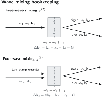
Energy and momentum bookkeeping for pair generation. A reciprocal-lattice or poling vector $\mathbf G$ allows quasi-phase matching. After replacing the strong pump mode or modes by classical amplitudes, both processes can reduce to the same two-mode squeezing Hamiltonian, but their pump scaling, selection rules, parasitic processes, and phase-matching conditions differ.

Energy and Momentum Matching

Longitudinal phase accumulation

Energy matching prevents rapid temporal phase winding. Spatial mode overlap must also add coherently along the device. For uniform collinear three-wave mixing, define

$$\Delta k = k_p-k_s-k_i-G,$$

where $G=0$ for ordinary phase matching and $G$ is a reciprocal poling vector for quasi-phase matching. The longitudinal amplitude contains

$$\begin{aligned} \int_0^L dz\,e^{i\Delta kz} ={}& L e^{i\Delta kL/2} \\ &\times \operatorname{sinc} \left( \frac{\Delta kL}{2} \right), \end{aligned}$$

where $\operatorname{sinc}x=\sin x/x$. The generated intensity or pair probability therefore carries

$$L^2 \operatorname{sinc}^2 \left( \frac{\Delta kL}{2} \right).$$

At exact phase matching, amplitudes from the full length add in phase. Away from it, longer interaction length narrows the acceptance bandwidth rather than indefinitely increasing useful output.

How phase matching is engineered

Common strategies include

• birefringent phase matching;
• periodic poling and higher-order quasi-phase matching;
• waveguide dispersion and transverse-mode engineering;
• cavity resonance matching;
• noncollinear geometry;
• temperature, strain, or electric-field tuning.

The vector equation also enforces transverse momentum or spatial-mode correlations. In a focused beam or a waveguide, replacing every mode by one plane-wave vector is an approximation; the full overlap integral is the reliable object.

Pump bandwidth and group velocity

For pulsed operation, the pump envelope constrains $\omega_s+\omega_i$ while the phase-matching function constrains a different combination of frequencies. Group-velocity mismatch tilts and narrows these constraints. Their product determines the joint spectral amplitude of a pair source.

Energy matching alone therefore does not determine the state. Two sources with the same central frequencies and brightness may have very different spectral entanglement, heralded purity, timing correlations, and collection efficiency.

Parametric Amplification

Undepleted-pump approximation

If the pump is bright and changes negligibly during the interaction, replace its operator by a coherent amplitude,

$$a_p \longrightarrow \alpha_p.$$

After moving to resonant rotating frames, the three-mode Hamiltonian becomes the two-mode squeezing interaction

$$\begin{aligned} H_{\rm 2sq} &= i\hbar \left( \xi a_s^\dagger a_i^\dagger - \xi^*a_s a_i \right), \\ \xi &= \kappa\alpha_p. \end{aligned}$$

This approximation removes pump depletion, pump quantum fluctuations, and pump-output entanglement. It is excellent when conversion is a negligible fraction of a stable pump and fails near strong depletion, oscillation threshold, or few-pump-photon operation.

For constant $\xi=|\xi|e^{i\phi}$ over an effective interaction time $t$, define $r=|\xi|t$. The Heisenberg transformation is

$$\begin{aligned} a_{s,\rm out} ={}& \cosh r\,a_{s,\rm in} + e^{i\phi}\sinh r\,a_{i,\rm in}^\dagger, \\ a_{i,\rm out} ={}& \cosh r\,a_{i,\rm in} + e^{i\phi}\sinh r\,a_{s,\rm in}^\dagger. \end{aligned}$$

The identity

$$\cosh^2r-\sinh^2r=1$$

preserves bosonic commutators. Omitting the conjugated idler term would appear to amplify a mode but would violate $[a_{\rm out},a_{\rm out}^\dagger]=1$.

Vacuum-seeded output

With both inputs in vacuum,

$$\langle n_s\rangle = \langle n_i\rangle = \sinh^2r.$$

The source has zero mean field, $\langle a_s\rangle=\langle a_i\rangle=0$, but nonzero occupation and pair correlation. Vacuum is not a hidden classical seed; it is the input quantum state whose fluctuations are transformed by the interaction.

The exact ideal output is

$$|\psi_{\rm 2sq}\rangle = \frac1{\cosh r} \sum_{n=0}^{\infty} \left( e^{i\phi}\tanh r \right)^n |n\rangle_s|n\rangle_i.$$

Signal and idler photon numbers are equal term by term. Either mode alone is thermal, while the joint state is pure and entangled for $r>0$.

Seeded phase-preserving gain

Let the idler input be vacuum and seed the signal without signal-idler correlations. With power gain

$$G=\cosh^2r,$$

the output signal occupation is

$$\langle n_{s,\rm out}\rangle = G\langle n_{s,\rm in}\rangle + (G-1).$$

The final term is spontaneous amplifier noise. A phase-preserving amplifier must treat both signal quadratures equally and requires an independent idler degree of freedom; at high gain, an ideal linear amplifier adds at least the equivalent of half a quantum when noise is referred to its input. Real loss or a thermally occupied idler raises that floor.

Degenerate phase-sensitive gain

If signal and idler are the same mode, the Hamiltonian is

$$H_{\rm 1sq} = \frac{i\hbar}{2} \left( \xi a^{\dagger2} - \xi^*a^2 \right).$$

With

$$X_\theta = \frac{ ae^{-i\theta} + a^\dagger e^{i\theta} }{ \sqrt2 },$$

an appropriate pair of orthogonal quadratures transforms as

$$\begin{aligned} X_{\phi/2,\rm out} &= e^rX_{\phi/2,\rm in}, \\ X_{\phi/2+\pi/2,\rm out} &= e^{-r}X_{\phi/2+\pi/2,\rm in}. \end{aligned}$$

One quadrature is amplified and the other deamplified. This ideal phase-sensitive amplifier need not add noise to the amplified quadrature, but it requires a phase reference and does not amplify an unknown phase equally. Squeezed Light owns the state, quadrature, decibel, loss, and verification conventions.

Resonators and threshold

A resonator increases interaction time and selects modes. For an ideal degenerate mode with energy-decay rate $\kappa_c$, a linearized equation has the form

$$\dot a = - \frac{\kappa_c}{2}a + \xi a^\dagger + \sqrt{\kappa_c}\,a_{\rm in}.$$

The small-signal threshold occurs at $|\xi|=\kappa_c/2$ in this convention. Below threshold, the device is an optical parametric amplifier or oscillator source of squeezed output. At threshold, the linearized gain diverges mathematically, signaling the failure of the undepleted-pump approximation. Above threshold, pump depletion and nonlinear saturation establish a finite oscillating field.

Frequency Conversion Is a Different Interaction

A strong pump can select a number-conserving difference-frequency term rather than pair creation:

$$H_{\rm fc} = \hbar \left( G_{\rm fc}a_b^\dagger a_a + G_{\rm fc}^*a_a^\dagger a_b \right).$$

This is an $SU(2)$ beam-splitter rotation in frequency space. For constant $G_{\rm fc}$,

$$\begin{aligned} a_{a,\rm out} &= \cos\vartheta\,a_{a,\rm in} - ie^{-i\varphi} \sin\vartheta\,a_{b,\rm in}, \\ a_{b,\rm out} &= \cos\vartheta\,a_{b,\rm in} - ie^{i\varphi} \sin\vartheta\,a_{a,\rm in}, \end{aligned}$$

where $\vartheta=|G_{\rm fc}|t$ and $\varphi=\arg G_{\rm fc}$. The conversion probability is $\sin^2\vartheta$.

Unlike a two-mode squeezer, this interaction preserves $n_a+n_b$ and cannot create photons from vacuum. It can translate a single-photon wavepacket, squeezed state, or entanglement between frequency bands if noise and mode mismatch are controlled.

χ³ Processes

Four-wave mixing

A third-order medium supports interactions among four waves. For two pump modes and signal-idler generation, a representative quantum Hamiltonian is

$$\begin{aligned} H_4 = i\hbar \Big( &\lambda a_{p1}a_{p2} a_s^\dagger a_i^\dagger \\ &- \lambda^* a_{p1}^\dagger a_{p2}^\dagger a_s a_i \Big). \end{aligned}$$

Replacing the pumps by classical amplitudes gives the same two-mode squeezing form as parametric down-conversion, with

$$\xi = \lambda\alpha_{p1}\alpha_{p2}.$$

For a single degenerate pump,

$$\begin{aligned} 2\omega_p &\simeq \omega_s+\omega_i, \\ \Delta k &= 2k_p-k_s-k_i-G. \end{aligned}$$

Self- and cross-phase modulation can add intensity-dependent contributions to the actual phase mismatch. A source model that includes pair generation but omits those shifts can predict the wrong bandwidth or optimum pump power.

Four-wave mixing is used in fibers, integrated waveguides, atomic vapors, microresonators, and superconducting circuits. Its desired pair process may compete with Raman scattering, fluorescence, pump leakage, two-photon absorption, free-carrier effects, or thermal noise. Those backgrounds do not share one universal scaling law, so they must be measured rather than folded into an unexplained “efficiency.”

Self-phase modulation and the Kerr Hamiltonian

Projecting a dispersive third-order response onto one ideal mode gives the Kerr Hamiltonian

$$\begin{aligned} H_{\rm K} &= \frac{\hbar K}{2} a^{\dagger2}a^2 \\ &= \frac{\hbar K}{2} n(n-1). \end{aligned}$$

Each Fock component acquires a number-dependent phase,

$$|n\rangle \longmapsto \exp\left[ - \frac{iKt}{2} n(n-1) \right] |n\rangle.$$

A coherent state therefore does not merely rotate rigidly in phase space: its different number components shear, producing quadrature squeezing at short times and non-Gaussian interference at special longer times. Loss rapidly erases the fine phase-space structure.

For two modes, an ideal cross-Kerr interaction is

$$H_{\rm X} = \hbar\chi_{\rm X}n_an_b.$$

It produces a phase in one mode conditioned on occupation of the other. This compact Hamiltonian is useful in resonators and effective circuit models, but a large clean single-photon cross-phase shift is difficult in a broadband traveling medium. Causality, finite response time, spectral entanglement, absorption, and Langevin noise must be included before claiming a deterministic photonic controlled phase.

Other third-order effects

The same $\chi^{(3)}$ family includes

• third-harmonic generation;
• self- and cross-phase modulation;
• modulation instability;
• four-wave-mixing amplification and wavelength conversion;
• spontaneous four-wave-mixing pair generation;
• frequency-comb formation in driven resonators.

The selected operator term depends on carrier frequencies, phase matching, pump configuration, and rotating frame. A classical label such as “self-phase modulation” does not specify the quantum noise model.

Multimode Pair Generation

A real traveling-wave source creates continua of signal and idler modes. In the low-gain regime, a generic interaction is

$$\begin{aligned} H_{\rm pair} &\simeq i\hbar \int d\omega_s\,d\omega_i \\ &\quad\times \Big[ F(\omega_s,\omega_i) a_s^\dagger(\omega_s) \\ &\qquad\times a_i^\dagger(\omega_i) - \text{H.c.} \Big]. \end{aligned}$$

The joint amplitude has the schematic structure

$$\begin{aligned} F(\omega_s,\omega_i) &\propto \alpha_p(\omega_s+\omega_i) \\ &\quad\times \Phi(\omega_s,\omega_i) \mathcal M(\omega_s,\omega_i), \end{aligned}$$

where $\alpha_p$ is the pump envelope, $\Phi$ the phase-matching function, and $\mathcal M$ collects spatial, polarization, and collection-mode overlaps.

A Schmidt decomposition writes the normalized amplitude as

$$\begin{aligned} F(\omega_s,\omega_i) &= \sum_k \sqrt{\lambda_k}\, u_k(\omega_s) \\ &\qquad\times v_k(\omega_i), \\ \sum_k\lambda_k &= 1. \end{aligned}$$

The effective spectral-mode number is

$$K_{\rm Sch} = \frac1{\sum_k\lambda_k^2}.$$

$K_{\rm Sch}=1$ corresponds to a factorable pair amplitude and permits a pure heralded photon in the ideal lossless, perfectly resolved limit. Filtering can reduce the accepted Schmidt number but usually sacrifices rate and heralding efficiency. Source engineering aims to shape pump and phase matching before detection rather than discarding most of the state afterward.

Quantum-State Generation Map

Pair creation

At low gain, two-mode squeezing gives

$$|\psi\rangle \simeq |0,0\rangle + \zeta|1,1\rangle + \zeta^2|2,2\rangle + \cdots.$$

Detecting one idler photon can herald a signal photon. Raising pump power increases the desired one-pair rate but also increases multipair contamination. A threshold detector that cannot distinguish one from two idler photons does not project onto an exact one-photon signal state.

Pair correlation is not automatically entanglement in every degree of freedom. The claimed subsystem, mode basis, density operator, and witness must be specified.

Gaussian state generation

Quadratic Hamiltonians in $a$ and $a^\dagger$ generate Gaussian unitaries:

• degenerate pair creation generates single-mode squeezing;
• nondegenerate pair creation generates two-mode squeezing and entanglement;
• frequency conversion implements a passive beam-splitter rotation;
• displacements supplied by coherent drives change first moments.

Gaussian unitaries acting on Gaussian inputs do not create Wigner negativity. Non-Gaussian resources require, for example, photon counting and conditioning, a sufficiently strong Kerr interaction, a discrete emitter, or a non-Gaussian input state.

Number-dependent phases

Kerr evolution is nonlinear in number operators and can generate non-Gaussian states from coherent light. The same sensitivity that makes it useful also makes it vulnerable: uncertainty in interaction time, loss, and photon number becomes phase noise.

Quantum frequency interfaces

Number-conserving conversion can connect wavelengths suited to memories, fiber transmission, detection, or microwave-to-optical interfaces. The conversion efficiency alone is not enough. A quantum interface should also report added noise, bandwidth, temporal-mode fidelity, pump leakage, and preservation of entanglement or nonclassical correlations.

Loss, Noise, and Open-System Completion

Loss is not merely a final reduction in count rate. It can

• mix vacuum or thermal noise into squeezed quadratures;
• destroy pair-number correlations asymmetrically;
• reduce heralding efficiency;
• make the surviving heralded state mixed;
• compete with coherent buildup inside a resonator;
• remove photons during Kerr evolution and randomize conditional phase.

An absorptive susceptibility must be accompanied by reservoir operators so output commutators remain correct. In a waveguide, distributed loss can act before, during, and after pair creation; replacing it by one beam splitter at the output is accurate only under stated conditions.

Useful measurements live on neighboring pages:

• Photon Counting owns detector POVMs, efficiency, dark counts, dead time, and number resolution.
• Correlation Functions owns $g^{(2)}$, cross-correlation, and mode-normalization conventions.
• Homodyne and Heterodyne Detection owns quadrature receivers and vacuum calibration.
• Input–Output Theory Overview owns resonator ports, linewidths, reflection, transmission, and collected output fields.

A Reliable Modeling Workflow

1. Declare the modes. Specify spatial profile, polarization, carrier, bandwidth, and normalization.
2. Identify the response. State the tensor component, frequency arguments, material symmetry, and whether absorption matters.
3. Choose pumps and quantum modes. Say which fields are operators and which are classical amplitudes.
4. Select rotating-wave terms. Check energy mismatch and identify pair creation, conversion, or Kerr evolution explicitly.
5. Evaluate overlap and phase matching. Include finite length, focusing, transverse structure, dispersion, and quasi-phase matching.
6. Test pump assumptions. Estimate depletion, gain, cavity threshold, and pump-noise transfer.
7. Add loss and parasitic processes. Include the noise operators required by dissipation.
8. Propagate to measured modes. Apply collection, filtering, propagation, detector response, and conditioning.
9. Report source and detected quantities separately. Internal generation probability, escape efficiency, heralding efficiency, and click rate are not interchangeable.

Common Mistakes

• Treating $\chi^{(m)}$ as a scalar constant. It is generally a dispersive tensor with symmetry, polarization, and absorption structure.
• Using energy conservation as the whole phase-matching condition. Spatial phases and mode overlap decide whether amplitudes add.
• Calling every $\chi^{(2)}$ device a down-converter. The selected frequencies and occupied inputs determine amplification, conversion, or harmonic generation.
• Replacing the pump by a number without checking depletion. The approximation also discards pump fluctuations and pump-output entanglement.
• Dropping the idler from an amplifier. Its conjugated operator preserves commutators and carries the minimum phase-preserving noise.
• Equating frequency conversion with amplification. Conversion is an $SU(2)$ number-conserving rotation; pair amplification is an $SU(1,1)$ transformation.
• Calling pair correlation entanglement. Classical mixtures can be correlated; an entanglement claim requires a state model and witness.
• Ignoring multimode structure. A single-mode Hamiltonian can fit total brightness while predicting the wrong heralded purity or homodyne mode.
• Treating loss as only fewer counts. Loss changes states, correlations, squeezing, and conditional purity.
• Assuming a large classical Kerr shift gives an ideal photonic gate. Response time, absorption, spectral entanglement, and noise can dominate at the single-photon level.

Exercises

Exercise 1: Inversion symmetry and an induced second-order response

In a scalar model,

$$\begin{aligned} P(E) &= \epsilon_0 \Big( \chi^{(1)}E + \chi^{(2)}E^2 \\ &\qquad + \chi^{(3)}E^3 + \cdots \Big). \end{aligned}$$

1. Show that inversion symmetry forces every even-order coefficient to vanish.
2. Suppose the centrosymmetric medium has a static bias $E_0$ and a small optical field $e(t)$, so $E=E_0+e$. Find the effective coefficient of $e^2$ generated by the $\chi^{(3)}E^3$ term.

Solution

Inversion symmetry requires

$$P(-E)=-P(E).$$

The polarization must therefore be an odd function of $E$. Comparing the series term by term gives

$$\chi^{(2)} = \chi^{(4)} = \cdots =0$$

for the ideal bulk electric-dipole response.

With a static bias,

$$\begin{aligned} \chi^{(3)}(E_0+e)^3 ={}& \chi^{(3)} \Big( E_0^3 + 3E_0^2e \\ &+ 3E_0e^2 + e^3 \Big). \end{aligned}$$

The term quadratic in the optical field is $3\chi^{(3)}E_0e^2$. In this scalar convention,

$$\chi_{\rm eff}^{(2)} = 3\chi^{(3)}E_0.$$

The tensor result depends on the bias direction and contracted indices. This is the electric-field-induced second-harmonic mechanism in its simplest form.

Exercise 2: Finite-length phase matching

A uniform waveguide has length $L=20\ \mathrm{mm}$ and constant phase mismatch $\Delta k=100\ \mathrm{m^{-1}}$.

1. Find the generated intensity relative to exact phase matching, using only the longitudinal $\operatorname{sinc}^2$ factor.
2. Find the magnitude of the first nonzero $\Delta k$ for which the longitudinal amplitude vanishes.

Solution

The dimensionless argument is

$$x = \frac{\Delta kL}{2} = \frac{ (100\ \mathrm{m^{-1}}) (0.020\ \mathrm m) }{2} =1.$$

Therefore

$$\frac{I(\Delta k)}{I(0)} = \operatorname{sinc}^2(1) = \left( \frac{\sin1}{1} \right)^2 \simeq 0.708.$$

The first zero occurs when

$$\frac{|\Delta k|L}{2} = \pi,$$

so

$$|\Delta k|_{\rm zero} = \frac{2\pi}{L} \simeq 314\ \mathrm{m^{-1}}.$$

A longer device raises the exactly matched amplitude but narrows the accepted mismatch range.

Exercise 3: One pump quantum in a three-wave mixer

Take real $\kappa>0$ and

$$H_3 = i\hbar\kappa \left( a_pa_s^\dagger a_i^\dagger - a_p^\dagger a_sa_i \right).$$

Start in $|1,0,0\rangle_{p,s,i}$.

1. Show that evolution remains in the span of $|1,0,0\rangle$ and $|0,1,1\rangle$.
2. Find the exact state and conversion probability.
3. Verify the Manley–Rowe invariants.

Solution

The Hamiltonian acts as

$$\begin{aligned} H_3|1,0,0\rangle &= i\hbar\kappa|0,1,1\rangle, \\ H_3|0,1,1\rangle &= -i\hbar\kappa|1,0,0\rangle. \end{aligned}$$

No other state is connected because there is at most one pump quantum and one signal-idler pair. Exponentiating this two-state generator gives

$$\begin{aligned} |\psi(t)\rangle ={}& \cos(\kappa t)|1,0,0\rangle \\ &+ \sin(\kappa t)|0,1,1\rangle. \end{aligned}$$

Thus

$$P_{\rm pair}(t) = \sin^2(\kappa t).$$

Both basis states have

$$\begin{gathered} n_p+n_s=1, \qquad n_p+n_i=1, \\ n_s-n_i=0. \end{gathered}$$

Every superposition in the invariant subspace has the same eigenvalues of those three combinations.

Exercise 4: Gain and spontaneous amplifier output

A nondegenerate parametric amplifier has $r=0.8$. Its idler input is vacuum, and its signal input has mean occupation $4$ with no signal-idler correlation.

1. Find the power gain $G$.
2. Find the output signal and idler occupations.
3. Verify that their mean difference equals the input signal-idler difference.

Solution

The gain is

$$G = \cosh^2(0.8) \simeq 1.789,$$

and

$$G-1 = \sinh^2(0.8) \simeq 0.789.$$

For a vacuum idler,

$$\begin{aligned} \langle n_{s,\rm out}\rangle &= G(4)+(G-1) \simeq 7.94, \\ \langle n_{i,\rm out}\rangle &= (G-1)(4+1) \simeq 3.94. \end{aligned}$$

Their difference is

$$\langle n_{s,\rm out}-n_{i,\rm out}\rangle \simeq 4.00,$$

equal to its input value. The added photons appear as pairs, preserving $n_s-n_i$.

Exercise 5: Squeezing followed by loss

A degenerate parametric interaction produces $r=0.7$ from vacuum, using the quadrature convention $V_{\rm vac}=1/2$. The squeezed mode then passes through an efficiency $\eta=0.80$ channel.

1. Find the ideal squeezed and anti-squeezed variances.
2. Find the observed squeezed variance.
3. Express the observed squeezing in decibels relative to vacuum.

Solution

The ideal variances are

$$\begin{aligned} V_{\min} &= \frac12e^{-2r} = \frac12e^{-1.4} \simeq 0.123, \\ V_{\max} &= \frac12e^{2r} = \frac12e^{1.4} \simeq 2.03. \end{aligned}$$

Loss mixes in vacuum:

$$\begin{aligned} V_{\rm obs} &= \eta V_{\min} + (1-\eta)\frac12 \\ &= (0.80)(0.123) + (0.20)(0.5) \\ &\simeq 0.199. \end{aligned}$$

Relative to vacuum,

$$\begin{aligned} S_{\rm dB} &= 10\log_{10} \left( \frac{V_{\rm obs}}{1/2} \right) \\ &\simeq 10\log_{10}(0.397) \simeq -4.01\ \mathrm{dB}. \end{aligned}$$

The source produced about $-6.08\ \mathrm{dB}$ ideally, but $20\%$ loss reduced the directly observed squeezing.

Exercise 6: Single-photon frequency conversion

A frequency converter has mixing angle $\vartheta=\pi/3$ and pump phase $\varphi=0$. It acts on an input $|1\rangle_a|0\rangle_b$.

1. Find the output state.
2. Find the conversion probability.
3. Explain what happens to vacuum input.

Solution

The creation-operator transformation gives

$$|1,0\rangle \longmapsto \cos\vartheta\,|1,0\rangle - i\sin\vartheta\,|0,1\rangle.$$

At $\vartheta=\pi/3$,

$$|\psi_{\rm out}\rangle = \frac12|1,0\rangle - i\frac{\sqrt3}{2}|0,1\rangle.$$

The conversion probability is

$$P_{a\to b} = \sin^2\left(\frac{\pi}{3}\right) = \frac34.$$

The two-mode vacuum remains vacuum because the interaction conserves total photon number. This is a coherent frequency beam splitter, not a vacuum-seeded amplifier.

Exercise 7: Kerr phases are not a rigid rotation

The initial state is

$$|\psi(0)\rangle = \frac{ |0\rangle+|1\rangle+|2\rangle }{ \sqrt3 }.$$

It evolves under

$$H_{\rm K} = \frac{\hbar K}{2}n(n-1)$$

for a time $Kt=\pi$.

1. Find the final state.
2. Compare $\langle n\rangle$ before and after.
3. Compare $\langle a\rangle$ before and after.

Solution

The phases for $n=0,1,2$ are respectively

$$1,\qquad 1,\qquad e^{-i\pi}=-1.$$

Therefore

$$|\psi(t)\rangle = \frac{ |0\rangle+|1\rangle-|2\rangle }{ \sqrt3 }.$$

The number probabilities are unchanged, so

$$\langle n\rangle = \frac{0+1+2}{3} =1$$

both before and after. Initially,

$$\langle a\rangle_0 = \frac{1+\sqrt2}{3},$$

whereas afterward,

$$\langle a\rangle_t = \frac{1-\sqrt2}{3}.$$

Kerr evolution preserves number while changing relative phases between number sectors. A rigid phase-space rotation would instead multiply $\langle a\rangle$ by a unit-modulus phase without changing its magnitude.

Exercise 8: Compare second- and third-order pump scaling

A selected low-gain second-order pair process has

$$\xi_2=\kappa_2\alpha_p,$$

while degenerate-pump four-wave mixing has

$$\xi_3=\kappa_3\alpha_p^2.$$

Assume pump power satisfies $P\propto|\alpha_p|^2$ and hold all other parameters fixed.

1. Find the low-gain pair-probability scaling with $P$ for each process.
2. By what factor does each probability change when the pump power doubles?
3. Give two reasons the simple power laws can fail experimentally.

Solution

At low gain, pair probability is proportional to squared interaction amplitude. Therefore

$$\begin{aligned} p_2 &\propto |\xi_2|^2 \propto |\alpha_p|^2 \propto P, \\ p_3 &\propto |\xi_3|^2 \propto |\alpha_p|^4 \propto P^2. \end{aligned}$$

Doubling $P$ therefore gives

$$\begin{aligned} p_2(2P) &= 2p_2(P), \\ p_3(2P) &= 4p_3(P). \end{aligned}$$

The laws assume undepleted pumps, fixed mode overlap, and fixed phase matching. Pump depletion, self- and cross-phase modulation, thermal or photorefractive detuning, nonlinear absorption, Raman background, and detector saturation can all change the measured scaling.

References

1. J. A. Armstrong, N. Bloembergen, J. Ducuing, and P. S. Pershan, “Interactions between light waves in a nonlinear dielectric,” Physical Review 127, 1918–1939 (1962).
2. N. Bloembergen, Nonlinear Optics (W. A. Benjamin, 1965).
3. Y. R. Shen, The Principles of Nonlinear Optics (Wiley, 1984).
4. R. W. Boyd, Nonlinear Optics, 4th ed. (Academic Press, 2020).
5. D. C. Burnham and D. L. Weinberg, “Observation of simultaneity in parametric production of optical photon pairs,” Physical Review Letters 25, 84–87 (1970).
6. C. K. Hong and L. Mandel, “Theory of parametric frequency down conversion of light,” Physical Review A 31, 2409–2418 (1985).
7. C. M. Caves, “Quantum limits on noise in linear amplifiers,” Physical Review D 26, 1817–1839 (1982).
8. R. E. Slusher, L. W. Hollberg, B. Yurke, J. C. Mertz, and J. F. Valley, “Observation of squeezed states generated by four-wave mixing in an optical cavity,” Physical Review Letters 55, 2409–2412 (1985).
9. L.-A. Wu, H. J. Kimble, J. L. Hall, and H. Wu, “Generation of squeezed states by parametric down conversion,” Physical Review Letters 57, 2520–2523 (1986).
10. L. Mandel and E. Wolf, Optical Coherence and Quantum Optics (Cambridge University Press, 1995).
11. R. Loudon, The Quantum Theory of Light, 3rd ed. (Oxford University Press, 2000).
12. D. F. Walls and G. J. Milburn, Quantum Optics, 2nd ed. (Springer, 2008).
13. G. P. Agrawal, Nonlinear Fiber Optics, 6th ed. (Academic Press, 2019).
14. S. L. Braunstein and P. van Loock, “Quantum information with continuous variables,” Reviews of Modern Physics 77, 513–577 (2005).
15. C. Weedbrook et al., “Gaussian quantum information,” Reviews of Modern Physics 84, 621–669 (2012).
16. C. K. Law, I. A. Walmsley, and J. H. Eberly, “Continuous frequency entanglement: Effective finite Hilbert space and entropy control,” Physical Review Letters 84, 5304–5307 (2000).
17. M. G. Raymer and K. Srinivasan, “Manipulating the color and shape of single photons,” Physics Today 65(11), 32–37 (2012).
18. D. Klyshko, Photons and Nonlinear Optics (Gordon and Breach, 1988).