Squeezed Light

Squeezed light is an electromagnetic field whose fluctuations in one declared quadrature are smaller than the fluctuations of the corresponding vacuum mode. For a normalized mode with annihilation operator $\hat a$, define

$$\hat X_\theta = \frac{ \hat a e^{-i\theta} + \hat a^\dagger e^{i\theta} }{ \sqrt2 }.$$

The orthogonal quadrature is $\hat X_{\theta+\pi/2}$, and

$$\left[ \hat X_\theta, \hat X_{\theta+\pi/2} \right] = i.$$

Vacuum and coherent states have

$$\operatorname{Var}_0(X_\theta) = \frac12$$

for every $\theta$. The operational squeezing criterion in this convention is

$$\min_\theta \operatorname{Var}(X_\theta) \lt \frac12.$$

The word declared matters. Squeezing is always relative to a mode, a quadrature angle, a bandwidth, and a calibrated vacuum reference. It does not mean that every field observable is quieter, that the uncertainty principle has been evaded, or that every photon-counting statistic is sub-Poissonian.

For an ideal single-mode squeezed vacuum with squeezing strength $r$,

$$V_{\min} = \frac12e^{-2r}, \qquad V_{\max} = \frac12e^{2r},$$

so the uncertainty product remains

$$\sqrt{V_{\min}V_{\max}} = \frac12.$$

Squeezing redistributes quantum noise. The narrow quadrature is accompanied by an anti-squeezed quadrature, and optical loss or phase error mixes part of that larger fluctuation back into the measurement.

Canonical Scope

This page is the canonical home for the optical realization of quadrature squeezing:

• which field mode and quadrature are squeezed;
• how standard optical interactions realize the squeeze transformation;
• how balanced homodyne detection verifies it;
• how squeezing is reported in linear units and decibels;
• how loss, thermal noise, mode mismatch, and phase noise limit observations;
• why squeezing can improve a precision measurement only when the signal and noise geometry are aligned.

The underlying oscillator construction is introduced in Squeezed States: First Encounter. Gaussian States and Wigner Functions owns the general covariance-matrix and Wigner-function framework. Squeezed States as Entangled Modes owns the distinction between single-mode squeezing and two-mode entanglement. Squeezing owns the cross-platform metrological comparison: declared reference noise, signal response, readout direction, Fisher information, and matched loss model. Homodyne and Heterodyne Detection owns the practical balanced receiver, shot-noise calibration, mode selection, and tomography connection. The open-systems Homodyne Detection owns stochastic records and conditional state updates. Nonlinear Quantum Optics owns the susceptibility-to-Hamiltonian derivation, phase matching, parametric gain, and four-wave-mixing process map. Here those interactions appear only as preparation mechanisms for states whose quadratures are then characterized. Parametric Down-Conversion owns low-gain biphoton source design, heralding, and polarization or time-bin pair encodings.

What a trustworthy squeezing claim reports

At minimum, report:

1. the temporal, spectral, spatial, and polarization mode;
2. the quadrature convention and vacuum variance;
3. the squeezed angle or phase-reference convention;
4. the analysis frequency and measurement bandwidth;
5. the raw observed noise ratio;
6. any electronic-noise subtraction or loss correction;
7. total efficiency, mode overlap, and phase uncertainty;
8. anti-squeezing and uncertainty, not only the best squeezed value.

“Six decibels of squeezing” without these qualifiers is incomplete. It may refer to an inferred source state, a directly measured detector record, one Fourier sideband band, or a correction that depends sensitively on an efficiency model.

Optical Field Quadratures

A single optical mode behaves algebraically like one harmonic oscillator, but its quadratures are physical field amplitudes rather than particle coordinates. Choose

$$\hat X = \frac{ \hat a+\hat a^\dagger }{ \sqrt2 }, \qquad \hat P = \frac{ \hat a-\hat a^\dagger }{ i\sqrt2 }.$$

Then

$$\hat X_\theta = \hat X\cos\theta + \hat P\sin\theta,$$

and

$$\hat X_{\theta+\pi/2} = -\hat X\sin\theta + \hat P\cos\theta.$$

For a narrowband traveling mode, the positive-frequency electric field has the schematic form

$$\hat E^{(+)}(t) = \mathcal E \hat a e^{-i\omega t},$$

where $\mathcal E$ contains the mode normalization. Interference with a phase reference converts a chosen linear combination of $\hat E^{(+)}$ and $\hat E^{(-)}$ into $\hat X_\theta$. A quadrature is therefore not an independent polarization or a separate beam. It is a phase-selected component of one complex mode amplitude.

Equivalent normalizations

Three conventions are common:

$$\hat X = \frac{ \hat a+\hat a^\dagger }{ \sqrt2 }, \qquad \operatorname{Var}_0(X) = \frac12;$$ $$\hat x = \frac{ \hat a+\hat a^\dagger }{ 2 }, \qquad \operatorname{Var}_0(x) = \frac14;$$

and a noise-normalized convention with

$$v_\theta \equiv \frac{ \operatorname{Var}(X_\theta) }{ \operatorname{Var}_0(X_\theta) }, \qquad v_{\mathrm{vac}}=1.$$

All three describe the same physics. Problems arise only when a formula or plot is compared without converting its reference level. This page uses $\operatorname{Var}_0(X_\theta)=1/2$ for operators and $v_{\mathrm{vac}}=1$ for measured noise ratios.

Means versus fluctuations

Write the fluctuation operator as

$$\delta\hat X_\theta = \hat X_\theta - \langle\hat X_\theta\rangle.$$

Squeezing concerns

$$\operatorname{Var}(X_\theta) = \left\langle (\delta\hat X_\theta)^2 \right\rangle,$$

not the mean field. A squeezed vacuum has

$$\langle\hat a\rangle=0,$$

whereas a displaced squeezed state can be bright:

$$\langle\hat a\rangle=\alpha.$$

Both can have the same covariance ellipse. Conversely, a highly stable bright coherent beam has a large mean amplitude but vacuum-level quadrature fluctuations rather than squeezing.

Vacuum Reference and Decibels

The normalized quadrature noise is

$$v_\theta = 2\operatorname{Var}(X_\theta)$$

in the convention used here. Vacuum gives $v_\theta=1$, squeezing gives $v_\theta\lt1$, and anti-squeezing gives $v_\theta\gt1$.

Noise power relative to vacuum is often plotted as

$$L_\theta = 10\log_{10}v_\theta \ \mathrm{dB}.$$

Thus a squeezed trace lies at a negative value. Experimental prose often quotes a positive squeezing magnitude,

$$R_{\mathrm{sq}} = -10\log_{10}v_{\min} \ \mathrm{dB}.$$

For an ideal squeezed vacuum,

$$v_{\min}=e^{-2r}, \qquad v_{\max}=e^{2r},$$

so

$$R_{\mathrm{sq}} = \frac{ 20r }{ \ln 10 } \ \mathrm{dB} \approx 8.686r \ \mathrm{dB}.$$

Three decibels of squeezing means approximately half the variance:

$$10^{-3/10} \approx 0.501.$$

The corresponding standard deviation is smaller by approximately $1/\sqrt2$. Using $20\log_{10}$ directly on a variance double-counts the conversion.

Uncertainty Ellipse

For $\hat{\boldsymbol R}=(\hat X,\hat P)^{\mathsf T}$, define the covariance matrix

$$V_{jk} = \frac12 \left\langle \delta\hat R_j\delta\hat R_k + \delta\hat R_k\delta\hat R_j \right\rangle.$$

The variance along the unit vector

$$\boldsymbol u_\theta = \begin{pmatrix} \cos\theta\\ \sin\theta \end{pmatrix}$$

is

$$\operatorname{Var}(X_\theta) = \boldsymbol u_\theta^{\mathsf T} V \boldsymbol u_\theta.$$

The eigenvectors of $V$ are the principal quadrature axes. Its eigenvalues are $V_{\min}$ and $V_{\max}$. For one canonical mode, the uncertainty principle requires

$$\det V \ge \frac14.$$

An ideal pure squeezed vacuum saturates the bound. A mixed squeezed state can still satisfy $V_{\min}\lt1/2$ while having

$$\det V \gt \frac14.$$

Its ellipse has more area than the minimum-uncertainty ellipse.

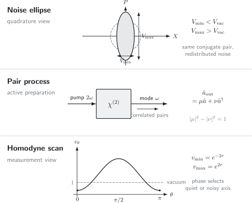
Squeezed light is a linked preparation-and-measurement statement. A nonlinear interaction reshapes vacuum fluctuations, the squeezed and anti-squeezed quadratures remain conjugate, and a phase-referenced homodyne scan reveals a noise minimum below the calibrated vacuum level.

Rotated ellipse

For a general symmetric covariance matrix,

$$V = \begin{pmatrix} V_{XX} & V_{XP}\\ V_{XP} & V_{PP} \end{pmatrix},$$

the principal-axis angle satisfies

$$\tan(2\theta_{\mathrm{sq}}) = \frac{ 2V_{XP} }{ V_{XX}-V_{PP} }.$$

The factor of two is characteristic of an ellipse: a rotation by $\pi$ returns the same quadrature axis. A squeezing phase and a local-oscillator phase must therefore be related with care; they are not always numerically the same angle.

Squeeze Operator and State Family

Let

$$\zeta = r e^{i\phi}, \qquad r\ge0.$$

One standard single-mode squeeze operator is

$$\hat S(\zeta) = \exp\left[ \frac12 \left( \zeta^*\hat a^2 - \zeta(\hat a^\dagger)^2 \right) \right].$$

It generates the squeezed vacuum

$$\lvert0;\zeta\rangle = \hat S(\zeta)\lvert0\rangle.$$

The corresponding Bogoliubov transformation is

$$\hat S^\dagger(\zeta) \hat a \hat S(\zeta) = \hat a\cosh r - e^{i\phi} \hat a^\dagger\sinh r.$$

The commutator is preserved because

$$\cosh^2r-\sinh^2r=1.$$

For the squeezed vacuum,

$$\begin{aligned} \operatorname{Var}(X_\theta) &= \frac12\cosh(2r) \\ &\quad - \frac12\sinh(2r) \cos(2\theta-\phi) . \end{aligned}$$

The minimum occurs at

$$\theta_{\mathrm{sq}} = \frac{\phi}{2} \pmod{\pi},$$

and the orthogonal quadrature is anti-squeezed:

$$\begin{aligned} \operatorname{Var}(X_{\theta_{\mathrm{sq}}}) &= \frac12e^{-2r}, \\ \operatorname{Var}(X_{\theta_{\mathrm{sq}}+\pi/2}) &= \frac12e^{2r}. \end{aligned}$$

Changing the sign convention in $\hat S$ shifts the quoted squeezing phase. The invariant content is the measured principal axis and its variance.

Displaced squeezed states

The displacement operator

$$\hat D(\alpha) = \exp\left( \alpha\hat a^\dagger - \alpha^*\hat a \right)$$

produces

$$\lvert\alpha,\zeta\rangle = \hat D(\alpha) \hat S(\zeta) \lvert0\rangle.$$

With this ordering,

$$\langle\hat a\rangle=\alpha,$$

while the covariance is that of the squeezed vacuum. The alternative order $\hat S(\zeta)\hat D(\alpha)$ represents the same family with a transformed displacement parameter, but it does not use the same numerical $\alpha$.

The relative angle between displacement and squeezing controls direct intensity fluctuations. An amplitude-squeezed bright state can be sub-Poissonian, while a phase-squeezed bright state can be super-Poissonian. Quadrature squeezing and sub-Poissonian counting are different witnesses of nonclassicality.

Squeezed thermal states

A useful mixed Gaussian model is

$$\rho_{\mathrm{sth}} = \hat S(\zeta) \rho_{\mathrm{th}} \hat S^\dagger(\zeta),$$

where the unsqueezed thermal mode has mean occupation $n_{\mathrm{th}}$. Along the principal axes,

$$\begin{aligned} V_{\min} &= \left( n_{\mathrm{th}}+\frac12 \right) e^{-2r}, \\ V_{\max} &= \left( n_{\mathrm{th}}+\frac12 \right) e^{2r}. \end{aligned}$$

The state is squeezed below vacuum only if

$$(2n_{\mathrm{th}}+1)e^{-2r} \lt 1.$$

Its covariance determinant is

$$\det V = \left( n_{\mathrm{th}}+\frac12 \right)^2,$$

and its purity is

$$\operatorname{Tr}(\rho_{\mathrm{sth}}^2) = \frac1{2n_{\mathrm{th}}+1}.$$

Parametric gain can create a visibly elongated ellipse without pushing the narrow axis below vacuum when the input or environment is too noisy. “Phase-sensitive amplification” is therefore broader than “generation of nonclassical squeezed light.”

Number-state signature

The squeezed vacuum contains only even photon numbers. Its mean occupation is

$$\bar n = \sinh^2r,$$

and its number variance is

$$\operatorname{Var}(N) = 2\bar n(\bar n+1).$$

Consequently,

$$g^{(2)}(0) = 3+\frac1{\bar n}.$$

The state is strongly super-Poissonian even though one quadrature is quieter than vacuum. This is not contradictory: photon number is not the squeezed quadrature. Photon Number States develops number-resolved diagnostics, while the oscillator page gives the canonical even-number expansion.

Nonclassical without Wigner negativity

The Wigner function of an ideal squeezed vacuum is a positive Gaussian. Yet a quadrature variance below vacuum is incompatible with an ordinary nonnegative Glauber–Sudarshan $P$ distribution. Squeezing is therefore a nonclassicality witness even when the Wigner function never becomes negative.

Wigner negativity is sufficient for nonclassicality, not necessary. This distinction is central when Gaussian resources are compared with photon-added, photon-subtracted, or number-state resources.

Which Optical Mode Is Squeezed?

The operator $\hat a$ must represent a normalized field mode. For a temporal or spectral wave packet,

$$\hat A_f = \int d\omega\, f^*(\omega) \hat a(\omega),$$

with

$$\int d\omega\, \lvert f(\omega)\rvert^2 = 1.$$

Then

$$[\hat A_f,\hat A_f^\dagger]=1.$$

The statement “the pulse is squeezed” means that a specified wave-packet mode $f$ has a sub-vacuum quadrature. A detector or local oscillator selecting a different mode $g$ observes only their overlap,

$$\mu = \int d\omega\, g^*(\omega)f(\omega),$$

with the orthogonal component entering as loss or added noise according to its state.

Continuous-wave sidebands

Continuous-wave squeezing is commonly reported at an analysis frequency $\Omega$ around a carrier $\omega_0$. The electronic photocurrent at $\Omega$ combines optical sidebands near

$$\omega_0+\Omega \qquad\text{and}\qquad \omega_0-\Omega.$$

A spectral quadrature is therefore generally a joint observable of the upper and lower sideband modes. Pair generation correlates those sidebands, and homodyne detection converts their correlation into sub-vacuum noise at the electronic analysis frequency.

Calling this “one monochromatic mode squeezed at $\omega_0$” hides important bookkeeping. A complete continuous-wave statement names:

• the optical carrier;
• the analysis sideband frequency;
• the resolution and video bandwidths;
• whether the noise spectrum is single-sided or double-sided;
• the temporal integration used to define the detected mode.

Multimode squeezing

A pulsed nonlinear interaction can have the schematic pair-creation kernel

$$\begin{aligned} \hat H_I &= i\hbar \iint d\omega\,d\omega'\, \hat{\mathcal K}(\omega,\omega'), \\ \hat{\mathcal K}(\omega,\omega') &= \kappa(\omega,\omega') \hat a^\dagger(\omega) \hat a^\dagger(\omega') \\ &\quad - \mathrm{h.c.} \end{aligned}$$

Pump bandwidth, dispersion, and phase matching determine $\kappa(\omega,\omega')$. In general, the output is not one uniformly squeezed pulse mode. A singular-mode or Bloch–Messiah decomposition identifies orthogonal supermodes with different squeezing strengths.

This matters experimentally. A local oscillator matched to the leading supermode can reveal strong squeezing, while an unmatched ultrashort pulse averages squeezed and unsqueezed modes. Mode Decompositions provides the broader tensor-factor bookkeeping.

Generation Mechanisms

Squeezing requires an active interaction that mixes annihilation and creation operators. Passive phase shifts and beam splitters rotate or redistribute existing squeezing but cannot create it from coherent states and vacuum. The material response, mode overlap, and validity of the undepleted-pump reduction are developed in Nonlinear Quantum Optics.

Degenerate parametric interaction

In a second-order nonlinear medium, a strong classical pump near $2\omega$ can drive the effective Hamiltonian

$$\hat H_I = \frac{i\hbar\kappa}{2} \left( e^{-i\phi_p}\hat a^2 - e^{i\phi_p}(\hat a^\dagger)^2 \right).$$

For interaction time $t$, the evolution is a squeeze operator with

$$r=\kappa t$$

in this ideal undepleted-pump model. The pump supplies energy and fixes the squeezing phase. At the operator level, the output has the general phase-sensitive form

$$\hat a_{\mathrm{out}} = \mu\hat a_{\mathrm{in}} + \nu\hat a_{\mathrm{in}}^\dagger,$$

where

$$\lvert\mu\rvert^2 - \lvert\nu\rvert^2 = 1.$$

One principal quadrature is deamplified while its conjugate is amplified. The vacuum seed is transformed into squeezed vacuum; a coherent seed becomes a displaced squeezed state.

Energy and momentum matching

For nondegenerate parametric down-conversion,

$$\omega_p = \omega_s+\omega_i.$$

Efficient conversion also requires phase matching, schematically

$$\boldsymbol k_p \approx \boldsymbol k_s+\boldsymbol k_i,$$

with a reciprocal-lattice contribution for quasi-phase matching. Degenerate squeezing sets $\omega_s=\omega_i=\omega_p/2$ but can still involve distinct spatial, polarization, or sideband modes.

The phrases degenerate, single-mode, and collinear answer different questions. Degenerate frequencies do not guarantee a single spatiotemporal mode, and a single beam can contain many independently squeezed supermodes.

Optical parametric oscillators

Placing the nonlinear medium in a cavity enhances the interaction and selects a frequency-dependent output mode. Below threshold, an optical parametric oscillator can emit squeezed vacuum with no coherent carrier in the squeezed port. Its useful description requires:

• cavity linewidth and escape efficiency;
• pump fraction relative to threshold;
• internal absorption and propagation loss;
• detuning and phase-lock errors;
• squeezing spectrum versus analysis frequency.

Approaching threshold increases ideal low-frequency squeezing and anti-squeezing, but it also increases sensitivity to phase noise, pump noise, and technical drift. Above threshold the device becomes an oscillator with a macroscopic signal, and the linearized state description must be rebuilt around that operating point.

Four-wave mixing

A third-order nonlinearity can drive

$$2\omega_p = \omega_s+\omega_i$$

through annihilation of two pump photons and correlated creation of signal and idler photons. Atomic vapors, optical fibers, integrated resonators, and other $\chi^{(3)}$ platforms can generate single-mode quadrature squeezing, twin-beam intensity-difference squeezing, or two-mode squeezing depending on the selected modes and pumps.

The first experimental observation of optical squeezing used four-wave mixing in an atomic cavity. The mechanism also introduces platform-specific noise: spontaneous emission, Raman scattering, pump leakage, absorption, and excess phase noise can obscure the ideal pair Hamiltonian.

Kerr shearing and emitter-based squeezing

A Kerr interaction proportional to

$$\hat H_{\mathrm K} \propto (\hat a^\dagger\hat a)^2$$

shears a coherent-state distribution in phase space. For suitable evolution and displacement, part of the sheared state can have reduced quadrature variance. At stronger evolution the state is non-Gaussian, so one ellipse no longer captures its full structure.

Resonance fluorescence and related driven-emitter fields can also display quadrature squeezing. Such sources are not equivalent to an ideal squeezed vacuum: their bandwidth, photon statistics, and non-Gaussian correlations are set by the emitter dynamics.

How Squeezing Is Measured

Quadrature squeezing is a phase-sensitive statement, so it requires a phase-sensitive measurement. Balanced homodyne detection is the standard reference method.

Balanced homodyne detection

Let $\hat a$ be the signal mode and $\hat b$ a strong coherent local-oscillator mode with

$$\beta = \lvert\beta\rvert e^{i\theta}.$$

A balanced beam splitter produces output modes

$$\hat c = \frac{ \hat a+\hat b }{ \sqrt2 }, \qquad \hat d = \frac{ \hat b-\hat a }{ \sqrt2 }.$$

The photon-number difference is

$$\hat N_c-\hat N_d = \hat a^\dagger\hat b + \hat b^\dagger\hat a.$$

For a strong local oscillator, replace $\hat b$ by $\beta$ in the leading signal term:

$$\hat N_c-\hat N_d \approx \sqrt2 \lvert\beta\rvert \hat X_\theta.$$

Changing the local-oscillator phase scans the quadrature angle. Balanced subtraction removes the large common local-oscillator intensity to first order and leaves a difference noise proportional to the signal quadrature variance.

The local oscillator does more than supply gain and phase. Its spatial, temporal, spectral, and polarization profile defines the measured mode. Excellent photodiodes cannot recover squeezing in a mode orthogonal to the local oscillator.

Establishing the vacuum level

A standard vacuum reference is obtained by blocking the signal before the homodyne beam splitter while keeping the local oscillator, detectors, electronic gain, filters, and analysis settings unchanged. The unused signal input then supplies vacuum fluctuations.

The measured difference-noise power should:

• scale linearly with local-oscillator optical power over the working range;
• remain well above electronic dark noise;
• stay below detector saturation and digitizer clipping;
• be stable under repeated vacuum–signal switching;
• be insensitive to classical common-mode local-oscillator noise after balancing.

A line labelled “shot noise” is not automatically a trustworthy vacuum calibration. Electronic noise subtraction, detector imbalance, resolution bandwidth, windowing, and spectral averaging all affect the displayed trace.

Spectral squeezing

For a stationary continuous-wave field, one measures a quadrature-noise power spectral density

$$S_{X_\theta X_\theta}(\Omega)$$

relative to the vacuum spectrum at analysis frequency $\Omega$. The result is often reported as

$$v_\theta(\Omega) = \frac{ S_{X_\theta X_\theta}(\Omega) }{ S_{\mathrm{vac}}(\Omega) }.$$

Squeezing can exist in one frequency band and disappear in another. A cavity source may be quantum-noise limited near its resonance yet dominated by pump, control, or acoustic noise at low analysis frequencies.

Comparisons require the same convention for:

• single-sided versus double-sided spectra;
• angular frequency versus ordinary frequency;
• power spectral density versus amplitude spectral density;
• raw spectrum-analyzer bins versus integrated mode variance.

A level in $\mathrm{dB}/\mathrm{Hz}$ is not the same object as a dimensionless single-mode variance until a temporal or spectral mode and integration rule have been supplied.

Direct detection answers a different question

Direct photon counting measures intensity or number statistics, not a phase-selected quadrature. An undisplaced squeezed vacuum has zero mean field, even-number support, and super-Poissonian number fluctuations. Its squeezing is therefore not revealed by asking whether its raw count variance is below a Poisson value.

A bright amplitude-squeezed beam can display sub-shot-noise intensity fluctuations, but that is a special alignment of displacement and covariance. Phase squeezing generally requires interferometric or homodyne conversion before it appears as an intensity signal.

Tomography versus witnessing

Observing one quadrature below vacuum witnesses nonclassicality for the measured mode under a trusted calibration. It does not reconstruct the full density operator.

Scanning many local-oscillator phases samples quadrature marginals and can support optical homodyne tomography. Reconstruction then requires a model for efficiency, phase sampling, finite statistics, and regularization. The general phase-space inversion belongs with Gaussian States and Wigner Functions and Phase-Space Distributions.

Loss and Added Noise

Loss is especially important for squeezing because vacuum entering an unobserved port fills in the narrow quadrature. Model pure loss of transmissivity $\eta$ as

$$\hat a_{\mathrm{out}} = \sqrt\eta\, \hat a_{\mathrm{in}} + \sqrt{1-\eta}\, \hat v,$$

where $\hat v$ is an independent vacuum mode. In vacuum-normalized units,

$$v_{\mathrm{out}} = \eta v_{\mathrm{in}} + (1-\eta).$$

For an ideal input squeezed vacuum,

$$\begin{aligned} v_{\min,\mathrm{out}} &= 1-\eta+\eta e^{-2r}, \\ v_{\max,\mathrm{out}} &= 1-\eta+\eta e^{2r}. \end{aligned}$$

Even infinite input squeezing cannot overcome the loss floor:

$$\lim_{r\to\infty} v_{\min,\mathrm{out}} = 1-\eta.$$

The corresponding best possible observed squeezing is

$$R_{\max} = -10\log_{10}(1-\eta) \ \mathrm{dB}.$$

For example, $\eta=0.90$ imposes a $10\ \mathrm{dB}$ ceiling even before phase noise or technical noise is included.

What belongs in the efficiency

A simple effective efficiency can combine independent vacuum-loss channels:

$$\eta_{\mathrm{tot}} = \eta_{\mathrm{esc}} \times \eta_{\mathrm{prop}} \times \eta_{\mathrm{vis}} \times \eta_{\mathrm{det}},$$

where the symbols may represent:

• source escape efficiency;
• propagation transmission;
• homodyne mode-overlap efficiency;
• photodiode quantum efficiency.

The mode-overlap factor is often the squared visibility after correcting for power imbalance. Multiplying efficiencies is valid only when each imperfection is well represented by independent mixing with vacuum. Stray coherent light, thermal background, electronic noise, or nonlinear detector response requires a different model.

Thermal or noisy environments

If the environment mode has mean occupation $n_{\mathrm{env}}$, the normalized quadrature variance becomes

$$v_{\mathrm{out}} = \eta v_{\mathrm{in}} + (1-\eta) \left( 2n_{\mathrm{env}}+1 \right).$$

This is a thermal-loss Gaussian channel. At optical frequencies, a laboratory environment is often effectively vacuum at the carrier frequency, but technical sidebands and control-field leakage need not be. At microwave frequencies, thermal occupation and amplifier-added noise are frequently central.

Gaussian Channels gives the canonical channel description. Calling every degradation “loss” can substantially overestimate the recoverable source squeezing.

Inferring source squeezing

Under a trusted pure-loss model,

$$v_{\mathrm{in}} = \frac{ v_{\mathrm{out}}-(1-\eta) }{ \eta }.$$

This inversion becomes ill-conditioned when the observed variance is near the loss floor or $\eta$ is uncertain. A mature result quotes the directly observed value first, then any inferred source value with propagated uncertainty and a stated channel model.

Phase Noise

Suppose the intended measurement axis is the squeezed principal quadrature, but the actual local-oscillator angle has error $\delta$. The measured normalized variance is

$$v(\delta) = e^{-2r}\cos^2\delta + e^{2r}\sin^2\delta.$$

For small $\delta$,

$$v(\delta) \approx e^{-2r} + \delta^2 \left( e^{2r}-e^{-2r} \right).$$

Large anti-squeezing makes even a small phase error costly. Increasing parametric gain can therefore make the observed minimum worse when phase control is not improved.

For zero-mean Gaussian phase jitter of variance $\sigma_\theta^2$, averaging over the angle gives

$$\overline v = \cosh(2r) - e^{-2\sigma_\theta^2} \sinh(2r).$$

With pure loss after the phase error,

$$v_{\mathrm{obs}} = 1-\eta + \eta\overline v.$$

Phase noise can arise from pump-phase fluctuations, local-oscillator drift, cavity-length noise, control sidebands, or a frequency-dependent rotation between source and detector.

Frequency-dependent angle

Dispersion and cavities can rotate the squeezing ellipse by an angle that depends on $\Omega$. This can be unwanted, or it can be engineered. A filter cavity deliberately rotates squeezed vacuum so that different quadratures are used in different frequency bands.

One homodyne phase cannot reveal the minimum at every analysis frequency when the ellipse rotates across the spectrum. Reporting only the best point can hide poor broadband performance.

Worked Example: Loss and Phase Error

Suppose a source produces ideal $10\ \mathrm{dB}$ squeezing:

$$v_{\min,\mathrm{in}}=0.10, \qquad v_{\max,\mathrm{in}}=10.$$

With total efficiency $\eta=0.80$ and perfect phase lock,

$$v_{\min,\mathrm{out}} = 0.20+0.80(0.10) = 0.28.$$

The directly observed squeezing is

$$-10\log_{10}(0.28) \approx 5.53\ \mathrm{dB}.$$

The observed anti-squeezing is

$$v_{\max,\mathrm{out}} = 0.20+0.80(10) = 8.20,$$

or about $9.14\ \mathrm{dB}$ above vacuum.

Now add a fixed phase error $\delta=2^\circ$. Before loss,

$$\begin{aligned} v(\delta) &= 0.10\cos^2(2^\circ) + 10\sin^2(2^\circ) \\ &\approx 0.112. \end{aligned}$$

After loss,

$$v_{\mathrm{obs}} \approx 0.20+0.80(0.112) \approx 0.290.$$

The observed squeezing falls to approximately $5.38\ \mathrm{dB}$. The phase penalty looks modest here, but it grows rapidly with anti-squeezing or phase jitter. This is why source gain, efficiency, and phase control must be optimized together.

Squeezing and Precision Measurement

Squeezing helps when a signal is encoded in a quadrature whose uncertainty has been reduced and when the anti-squeezed quadrature does not couple back into the estimator.

For a bright field with real displacement $\alpha$ and a small phase shift $\varphi$,

$$\langle\hat P\rangle \approx \sqrt2 \alpha\varphi.$$

Error propagation gives

$$\Delta\varphi \approx \frac{ \Delta P }{ \sqrt2\lvert\alpha\rvert }.$$

For coherent light,

$$\Delta P = \frac1{\sqrt2},$$

so

$$\Delta\varphi_{\mathrm{coh}} \approx \frac1{2\sqrt{\bar n}}, \qquad \bar n=\lvert\alpha\rvert^2.$$

If the phase quadrature is ideally squeezed by $r$,

$$\Delta\varphi_{\mathrm{sq}} \approx \frac{ e^{-r} }{ 2\sqrt{\bar n} }.$$

This local formula shows the noise advantage, but it is not a universal metrological bound. Fair resource accounting may need to include photons in the squeezed field, pump power, losses, estimator bias, bandwidth, and backaction.

Interferometer dark-port injection

Near a dark operating port, vacuum fluctuations entering the nominally unused input contribute to the output noise. Injecting squeezed vacuum into that port can reduce the measured quadrature noise without placing a bright carrier there. The squeezing angle must be aligned with the signal quadrature at the readout.

This strategy does not make all interferometer noise disappear:

• phase squeezing can reduce high-frequency photon-counting noise;
• the conjugate amplitude fluctuations can increase radiation-pressure backaction;
• optical loss replaces part of the injected state with ordinary vacuum;
• detuning and optomechanical response rotate the relevant quadrature with frequency.

Carlton Caves’s interferometer analysis made this tradeoff explicit and motivated squeezed-vacuum injection as a measurement resource.

Frequency-dependent squeezing in gravitational-wave detectors

Large interferometers need different quadrature orientations where photon-counting noise and radiation-pressure noise dominate. Filter cavities can rotate the injected squeezing angle across frequency so the same source reduces both contributions over a broad band.

This is an engineering achievement as much as a state-preparation result. Useful operation depends on low-loss optics, long-term phase and alignment control, stable filter-cavity detuning, and a detector-wide noise budget. Modern gravitational-wave observatories have demonstrated squeezed-light operation and frequency-dependent quantum-noise reduction, but the achieved astrophysical sensitivity is never determined by a squeezing number alone.

Other applications

Quadrature squeezing can support:

• displacement, force, and phase sensing;
• spectroscopy and absorption measurements;
• optical and microwave readout of mechanical or electrical systems;
• continuous-variable teleportation, dense coding, and cluster-state protocols;
• generation of two-mode entanglement by active interactions or passive mixing of appropriately oriented squeezed modes.

Each application has its own useful mode and noise observable. A source that performs well in narrowband homodyne detection may be poorly matched to a broadband pulsed protocol.

Single-Mode and Two-Mode Squeezing

Single-mode squeezing reduces one quadrature of one declared mode. It is not by itself bipartite entanglement because no subsystem split has been named.

Two-mode squeezing correlates modes $A$ and $B$. In one convention, collective quadratures such as

$$\hat X_A-\hat X_B \qquad\text{and}\qquad \hat P_A+\hat P_B$$

are squeezed. Each mode separately can have a thermal reduced state even though the joint state is pure and entangled.

A balanced beam splitter can convert two single-mode squeezed inputs with orthogonal squeezing angles into two-mode entanglement. Conversely, changing the mode basis can reveal single-mode squeezing hidden inside a multimode Gaussian state. The relevant statements depend on the physically declared mode decomposition, not only on a drawing of two beams.

The canonical derivation and entanglement criteria are in Squeezed States as Entangled Modes.

A Practical Verification Workflow

1. Define the mode

Specify carrier, sideband or pulse envelope, spatial profile, polarization, and integration time. State how the local oscillator or detector selects that mode.

2. Declare the quadrature units

Give the operator convention or state explicitly that vacuum noise is normalized to one. Distinguish variance, power spectral density, and amplitude spectral density.

3. Calibrate vacuum and electronics

Measure local-oscillator power scaling, detector linearity, dark noise, balance, and drift. Record whether electronic noise was subtracted and how its uncertainty was propagated.

4. Scan phase and frequency

Measure both the squeezed minimum and anti-squeezed maximum. Map the spectrum over the application band rather than reporting one favorable bin.

5. Build the loss and phase model

Separate source escape, propagation, mode overlap, detector efficiency, phase jitter, and non-vacuum added noise. Check whether an effective pure-loss description is actually justified.

6. Report observed and inferred quantities separately

Lead with the detector-plane noise ratio. If source squeezing is inferred, state the inversion, parameter uncertainties, and assumptions.

7. Test the application metric

Demonstrate improved estimator variance, signal-to-noise ratio, information rate, or task performance under a fair resource count. Squeezing at an unused angle or outside the signal bandwidth is not an operational advantage.

What Squeezed Light Is Not

Not a violation of uncertainty

The conjugate variance grows. Ideal pure squeezing preserves the minimum-uncertainty product; realistic squeezing usually enlarges it.

Not simply low intensity

Vacuum, a weak coherent state, and a weak squeezed vacuum can all have small mean photon number but very different fluctuations and correlations.

Not necessarily sub-Poissonian

Squeezed vacuum is super-Poissonian. Direct number squeezing requires a particular displacement and squeezing orientation.

Not necessarily Wigner-negative

Gaussian squeezed states have positive Wigner functions. Their sub-vacuum quadrature variance nevertheless makes their Glauber–Sudarshan description nonclassical.

Not automatically entangled

One squeezed mode has no bipartite entanglement until a subsystem decomposition is specified. Two-mode squeezing is a different operation.

Not specified by one decibel number

Squeezing is frequency-, mode-, phase-, and calibration-dependent. A source value inferred after loss correction is not the same as a directly observed application-band improvement.

Common Mistakes

Mixing quadrature conventions

Vacuum variance may be $1/2$, $1/4$, or one. Convert before comparing formulas or data.

Using the wrong logarithm factor

Variance and noise power use $10\log_{10}$. Standard deviation and field amplitude use $20\log_{10}$. They agree numerically only when the squared relation is handled consistently.

Ignoring anti-squeezing

A small phase error couples the anti-squeezed variance into the measured axis. Quoting only $V_{\min}$ hides this vulnerability.

Treating visibility as a cosmetic alignment number

Homodyne visibility determines mode overlap and therefore effective efficiency. Poor overlap mixes in an orthogonal mode.

Subtracting electronic noise without disclosure

Subtraction can make squeezing appear stronger and can become unstable when dark noise is comparable to shot noise. Report raw and corrected values.

Calling any phase-sensitive amplifier nonclassical

A thermal or technically noisy input can be deamplified along one axis without falling below vacuum. The vacuum reference is the nonclassical threshold.

Forgetting continuous-wave sidebands

A spectrum-analyzer point generally probes correlated upper and lower optical sidebands. It is not a literal photon-number measurement of one infinitely sharp carrier mode.

Equating squeezing with metrological advantage

Loss, backaction, resource counting, estimator choice, and unrelated technical noise can erase the practical gain.

Connections

• Nonlinear Quantum Optics derives the nonlinear mode couplings that act as squeeze operators and separates phase-sensitive amplification from frequency conversion.
• Parametric Down-Conversion develops the low-gain pair sectors, heralded states, and entanglement-source diagnostics of the same interaction.
• Phase-Space Distributions explains why squeezed Gaussian light can have a positive Wigner function while failing the positive-$P$ classicality criterion.
• Beam Splitters develops the passive two-mode rotation that redistributes quadratures and can convert suitable squeezed inputs into mode entanglement.
• Interferometers applies dark-port squeezing to a Mach–Zehnder phase estimator and makes the loss, angle-error, and resource assumptions explicit.
• Quantum Optics supplies the state–transformation–measurement map.
• Quantized Electromagnetic Modes fixes mode normalization and continuum conventions.
• Coherent Light provides the displaced-vacuum and shot-noise reference.
• Thermal Light contrasts isotropic classical Gaussian noise with anisotropic nonclassical squeezing.
• Squeezed States: First Encounter owns the introductory oscillator construction and uncertainty geometry.
• Squeezing develops the response-aware metrology criterion, covariance optimization, and the distinction between reduced noise and end-to-end precision gain.
• Gaussian States and Wigner Functions develops covariance matrices, purity, and phase-space evolution.
• Squeezed States as Entangled Modes develops two-mode squeezing and finite-energy EPR correlations.
• Homodyne Detection owns balanced-detection records and conditional state evolution.
• Gaussian Channels supplies loss, thermal noise, and added-noise channel language.
• Precision Measurement connects quantum noise to practical sensitivity and resource accounting.

Exercises

1. Rotated squeezed-vacuum variance

For $\zeta=re^{i\phi}$, use

$$\hat S^\dagger(\zeta) \hat a \hat S(\zeta) = \hat a\cosh r - e^{i\phi} \hat a^\dagger\sinh r$$

to derive

$$\begin{aligned} \operatorname{Var}(X_\theta) &= \frac12\cosh(2r) \\ &\quad - \frac12\sinh(2r) \cos(2\theta-\phi) . \end{aligned}$$

Find the squeezed angle, the two principal variances, and their product.

Solution

Transform the quadrature:

$$\begin{aligned} \hat B_\theta &= e^{-i\theta} \hat a\cosh r - e^{i(\phi-\theta)} \hat a^\dagger\sinh r \\ \hat S^\dagger \hat X_\theta \hat S &= \frac{ \hat B_\theta+\hat B_\theta^\dagger }{ \sqrt2 }. \end{aligned}$$

The vacuum mean vanishes. Using

$$\langle0\lvert \hat a\hat a^\dagger \rvert0\rangle = 1$$

and the vanishing of the other normally unordered quadratic vacuum moments gives

$$\begin{aligned} \operatorname{Var}(X_\theta) &= \frac12 \left( \cosh^2r+\sinh^2r \right) \\ &\quad - \cosh r\,\sinh r \cos(2\theta-\phi). \end{aligned}$$

Now use

$$\cosh^2r+\sinh^2r = \cosh(2r)$$

and

$$2\cosh r\,\sinh r = \sinh(2r)$$

to obtain the stated expression.

The minimum requires

$$\cos(2\theta-\phi)=1,$$

so

$$\theta_{\mathrm{sq}} = \frac{\phi}{2} \pmod{\pi}.$$

At that angle,

$$\begin{aligned} V_{\min} &= \frac12 \left[ \cosh(2r)-\sinh(2r) \right] \\ &= \frac12e^{-2r}. \end{aligned}$$

The orthogonal angle changes the cosine to $-1$:

$$V_{\max} = \frac12e^{2r}.$$

Therefore

$$V_{\min}V_{\max} = \frac14,$$

or

$$\Delta X_{\min} \Delta X_{\max} = \frac12.$$

The ideal squeezed vacuum remains a minimum-uncertainty state.

2. Convert squeezing between decibels and state parameters

An ideal squeezed vacuum is quoted as having $6.0\ \mathrm{dB}$ of squeezing. Find:

1. its normalized minimum variance;
2. its minimum standard deviation relative to vacuum;
3. the squeezing parameter $r$;
4. the mean photon number $\bar n=\sinh^2r$;
5. its ideal anti-squeezing in decibels.

Solution

The normalized variance is

$$v_{\min} = 10^{-6.0/10} \approx 0.251.$$

The standard-deviation ratio is

$$\frac{ \Delta X_{\min} }{ \Delta X_{\mathrm{vac}} } = \sqrt{v_{\min}} \approx 0.501.$$

For an ideal squeezed vacuum,

$$v_{\min}=e^{-2r},$$

so

$$r = -\frac12\ln v_{\min} \approx 0.691.$$

The mean occupation is

$$\bar n = \sinh^2(0.691) \approx 0.56.$$

Ideal squeezing has reciprocal principal variances:

$$v_{\max} = e^{2r} = \frac1{v_{\min}} \approx 3.98.$$

Thus the anti-squeezing is

$$10\log_{10}(v_{\max}) \approx +6.0\ \mathrm{dB}.$$

Real data need not have symmetric squeezing and anti-squeezing in decibels, because loss and excess noise enlarge the covariance determinant.

3. Loss floor and observed squeezing

A source produces $8.0\ \mathrm{dB}$ of ideal squeezing and is measured with total efficiency $\eta=0.75$.

1. Find the detector-plane normalized minimum variance.
2. Convert it to observed squeezing in decibels.
3. Find the maximum observable squeezing allowed by this efficiency even for an infinitely squeezed source.

Solution

The source variance is

$$v_{\mathrm{in}} = 10^{-8.0/10} \approx 0.1585.$$

Pure loss gives

$$\begin{aligned} v_{\mathrm{out}} &= 1-\eta+\eta v_{\mathrm{in}} \\ &= 0.25+0.75(0.1585) \\ &\approx 0.3689. \end{aligned}$$

The observed squeezing magnitude is

$$-10\log_{10}(0.3689) \approx 4.33\ \mathrm{dB}.$$

For infinite source squeezing,

$$v_{\mathrm{out}} \longrightarrow 1-\eta = 0.25.$$

The efficiency ceiling is therefore

$$R_{\max} = -10\log_{10}(0.25) \approx 6.02\ \mathrm{dB}.$$

No increase in source gain can move the detector below this floor under the assumed channel.

4. Leakage from the anti-squeezed quadrature

An ideal source has

$$v_{\min}=0.10, \qquad v_{\max}=10.$$

The homodyne angle is offset from the squeezed axis by $3^\circ$.

1. Find the variance before loss.
2. Find the variance and squeezing in decibels after efficiency $\eta=0.90$.
3. Explain why phase stability becomes more demanding as anti-squeezing increases.

Solution

At angle error $\delta$,

$$v(\delta) = v_{\min}\cos^2\delta + v_{\max}\sin^2\delta.$$

With $\delta=3^\circ$,

$$\begin{aligned} v(3^\circ) &= 0.10\cos^2(3^\circ) + 10\sin^2(3^\circ) \\ &\approx 0.127. \end{aligned}$$

After pure loss,

$$\begin{aligned} v_{\mathrm{obs}} &= 0.10+0.90(0.127) \\ &\approx 0.214. \end{aligned}$$

The observed squeezing is

$$-10\log_{10}(0.214) \approx 6.69\ \mathrm{dB}.$$

For small error,

$$v(\delta) \approx v_{\min} + \delta^2 \left( v_{\max}-v_{\min} \right).$$

The error coefficient grows approximately as $v_{\max}$. Raising the parametric gain narrows one axis but enlarges the noise available to leak from the orthogonal axis. Better intrinsic squeezing can therefore produce worse observed squeezing if the phase lock is not improved.

5. When is a squeezed thermal state below vacuum?

A mode begins in a thermal state with

$$n_{\mathrm{th}}=0.25$$

and is squeezed by $r=0.50$.

1. Find the minimum $r$ needed to cross below vacuum.
2. Find the normalized principal variances for $r=0.50$.
3. Find the squeezing in decibels and the state purity.

Solution

The normalized narrow-axis variance is

$$v_{\min} = (2n_{\mathrm{th}}+1)e^{-2r}.$$

Sub-vacuum noise requires

$$r \gt \frac12 \ln(2n_{\mathrm{th}}+1).$$

Here,

$$r_{\mathrm{threshold}} = \frac12\ln(1.5) \approx 0.203.$$

At $r=0.50$,

$$v_{\min} = 1.5e^{-1} \approx 0.552,$$

and

$$v_{\max} = 1.5e \approx 4.08.$$

The squeezed noise is

$$-10\log_{10}(0.552) \approx 2.58\ \mathrm{dB}$$

below vacuum. The purity is unchanged by the unitary squeeze operation:

$$\operatorname{Tr}(\rho^2) = \frac1{2n_{\mathrm{th}}+1} = \frac23.$$

The product

$$v_{\min}v_{\max} = (2n_{\mathrm{th}}+1)^2 = 2.25$$

also shows that the state is mixed rather than a minimum-uncertainty squeezed vacuum.

6. Photon bunching of squeezed vacuum

Use

$$\bar n = \langle N\rangle$$

and

$$\operatorname{Var}(N) = 2\bar n(\bar n+1)$$

to derive the equal-time intensity correlation

$$g^{(2)}(0) = \frac{ \langle N(N-1)\rangle }{ \bar n^2 }.$$

Interpret its low-occupation limit.

Solution

The factorial moment is related to the variance by

$$\langle N(N-1)\rangle = \operatorname{Var}(N) + \bar n^2 - \bar n.$$

Substitution gives

$$\begin{aligned} \langle N(N-1)\rangle &= 2\bar n(\bar n+1) + \bar n^2 - \bar n \\ &= 3\bar n^2+\bar n. \end{aligned}$$

Therefore

$$g^{(2)}(0) = 3+\frac1{\bar n}.$$

As $\bar n\to0$, the normalized correlation diverges. The squeezed vacuum is created in pairs, so conditioning on there being light strongly favors a two-photon contribution over two unrelated single-photon events. The absolute pair rate still tends to zero with the source brightness; a divergent normalized $g^{(2)}$ does not mean a large count rate.

This strong bunching coexists with quadrature squeezing because number and field quadrature are different observables.

7. Homodyne difference current and mode mismatch

For

$$\hat c = \frac{ \hat a+\hat b }{ \sqrt2 }, \qquad \hat d = \frac{ \hat b-\hat a }{ \sqrt2 },$$

derive $\hat N_c-\hat N_d$. Then take

$$\hat b\longrightarrow \lvert\beta\rvert e^{i\theta}$$

and identify the measured quadrature.

Finally, suppose the local oscillator overlaps the squeezed mode with efficiency $\eta_{\mathrm{mm}}$ and the orthogonal component is vacuum. Show that the normalized observed variance is

$$v_{\mathrm{obs}} = \eta_{\mathrm{mm}}v_{\mathrm{sq}} + (1-\eta_{\mathrm{mm}}).$$

Solution

Expanding the two output number operators gives

$$\begin{aligned} \hat N_c &= \frac12 \left( \hat a^\dagger\hat a + \hat a^\dagger\hat b + \hat b^\dagger\hat a + \hat b^\dagger\hat b \right), \\ \hat N_d &= \frac12 \left( \hat b^\dagger\hat b - \hat b^\dagger\hat a - \hat a^\dagger\hat b + \hat a^\dagger\hat a \right). \end{aligned}$$

Subtracting cancels the direct intensities:

$$\hat N_c-\hat N_d = \hat a^\dagger\hat b + \hat b^\dagger\hat a.$$

For a strong coherent local oscillator,

$$\begin{aligned} \hat N_c-\hat N_d &\approx \lvert\beta\rvert \left( \hat a^\dagger e^{i\theta} + \hat a e^{-i\theta} \right) \\ &= \sqrt2 \lvert\beta\rvert \hat X_\theta. \end{aligned}$$

Thus the local-oscillator phase selects the measured quadrature.

Represent the detected mode as a superposition of the desired squeezed mode and an orthogonal vacuum mode:

$$\hat A_{\mathrm{det}} = \sqrt{\eta_{\mathrm{mm}}} \hat A_{\mathrm{sq}} + \sqrt{1-\eta_{\mathrm{mm}}} \hat A_{\mathrm{vac}}.$$

The two modes are independent, so their quadrature variances add:

$$v_{\mathrm{obs}} = \eta_{\mathrm{mm}}v_{\mathrm{sq}} + (1-\eta_{\mathrm{mm}})v_{\mathrm{vac}}.$$

With $v_{\mathrm{vac}}=1$, this is the pure-loss formula. Mode mismatch is therefore a physical noise channel, not merely a reduction in displayed signal amplitude.

8. Interpret a continuous-wave squeezing measurement

A degenerate optical parametric oscillator is pumped near $2\omega_0$. A balanced homodyne detector uses a local oscillator at $\omega_0$, and a spectrum analyzer shows $4\ \mathrm{dB}$ noise reduction at electronic frequency $\Omega$.

Answer the following:

1. Which optical frequencies contribute to that spectral point?
2. Why is it incomplete to call the result “one monochromatic mode at $\omega_0$ squeezed”?
3. What additional information is needed to turn the trace into a reproducible squeezing claim?

Solution

The homodyne photocurrent at electronic frequency $\Omega$ combines optical sidebands near

$$\omega_0+\Omega \qquad\text{and}\qquad \omega_0-\Omega.$$

The parametric interaction creates correlations between those sidebands because their frequencies sum to approximately $2\omega_0$. The spectral quadrature measured at $\Omega$ is a joint sideband observable selected by the local oscillator and electronic filter.

Calling the carrier alone squeezed hides this two-sideband structure and the finite temporal mode defined by the analyzer bandwidth. An infinitely sharp mode at exactly $\omega_0$ is not what the finite-time detector samples.

A reproducible claim should also state:

• the optical carrier and local-oscillator mode;
• the analyzed quadrature phase;
• analysis frequency, resolution bandwidth, video bandwidth, and averaging;
• the vacuum and electronic-noise calibrations;
• single-sided or double-sided spectrum convention;
• detector efficiency, propagation loss, and homodyne visibility;
• whether $4\ \mathrm{dB}$ is raw at the detector or corrected to the source;
• the anti-squeezed trace and phase uncertainty.

The same source may show different squeezing at another $\Omega$ because of cavity response, dispersion, loss, or technical noise.

References

1. H. P. Yuen, “Two-Photon Coherent States of the Radiation Field,” Physical Review A 13, 2226–2243 (1976), doi:10.1103/PhysRevA.13.2226.
2. H. N. Hollenhorst, “Quantum Limits on Resonant-Mass Gravitational-Radiation Detectors,” Physical Review D 19, 1669–1679 (1979), doi:10.1103/PhysRevD.19.1669.
3. C. M. Caves, “Quantum-Mechanical Noise in an Interferometer,” Physical Review D 23, 1693–1708 (1981), doi:10.1103/PhysRevD.23.1693.
4. D. F. Walls, “Squeezed States of Light,” Nature 306, 141–146 (1983), doi:10.1038/306141a0.
5. R. E. Slusher, L. W. Hollberg, B. Yurke, J. C. Mertz, and J. F. Valley, “Observation of Squeezed States Generated by Four-Wave Mixing in an Optical Cavity,” Physical Review Letters 55, 2409–2412 (1985), doi:10.1103/PhysRevLett.55.2409.
6. L.-A. Wu, H. J. Kimble, J. L. Hall, and H. Wu, “Generation of Squeezed States by Parametric Down Conversion,” Physical Review Letters 57, 2520–2523 (1986), doi:10.1103/PhysRevLett.57.2520.
7. S. L. Braunstein and P. van Loock, “Quantum Information with Continuous Variables,” Reviews of Modern Physics 77, 513–577 (2005), doi:10.1103/RevModPhys.77.513.
8. D. F. Walls and G. J. Milburn, Quantum Optics, 2nd ed., Springer (2008), doi:10.1007/978-3-540-28574-8.
9. U. L. Andersen, G. Leuchs, and C. Silberhorn, “Continuous-Variable Quantum Information Processing,” Laser & Photonics Reviews 4, 337–354 (2010), doi:10.1002/lpor.200910010.
10. A. I. Lvovsky, “Squeezed Light,” in Photonics: Scientific Foundations, Technology and Applications, Vol. 1, Wiley (2015), doi:10.1002/9781119009719.ch5.
11. U. L. Andersen, T. Gehring, C. Marquardt, and G. Leuchs, “30 Years of Squeezed Light Generation,” Physica Scripta 91, 053001 (2016), doi:10.1088/0031-8949/91/5/053001.
12. H. Vahlbruch, M. Mehmet, K. Danzmann, and R. Schnabel, “Detection of 15 dB Squeezed States of Light and Their Application for the Absolute Calibration of Photoelectric Quantum Efficiency,” Physical Review Letters 117, 110801 (2016), doi:10.1103/PhysRevLett.117.110801.
13. R. Schnabel, “Squeezed States of Light and Their Applications in Laser Interferometers,” Physics Reports 684, 1–51 (2017), doi:10.1016/j.physrep.2017.04.001.
14. F. Acernese et al. (Virgo Collaboration), “Increasing the Astrophysical Reach of the Advanced Virgo Detector via the Application of Squeezed Vacuum States of Light,” Physical Review Letters 123, 231108 (2019), doi:10.1103/PhysRevLett.123.231108.
15. W. Jia et al. (LIGO Scientific Collaboration), “Squeezing the Quantum Noise of a Gravitational-Wave Detector below the Standard Quantum Limit,” Science 385, 1318–1321 (2024), doi:10.1126/science.ado8069.

Frontier Context

Quantum Optics Frontiers compares application-level squeezing, integrated continuous-variable circuits, non-Gaussian resource generation, and fault-tolerance claims. This page remains the canonical derivation and calibration guide for squeezed light.