Cavity QED

Cavity quantum electrodynamics studies the coherent and dissipative dynamics of quantum emitters coupled to selected electromagnetic resonances. A cavity does more than store light. It concentrates the electric field into a small mode volume, repeatedly brings that field past the emitter, and routes part of the emitted radiation into identifiable output channels. These three effects can make the interaction of one emitter with one photon measurable, controllable, and sometimes faster than every relevant loss process.

The smallest useful model contains one cavity mode, one optical transition, and several reservoirs. Its behavior is governed not by the coupling $g$ alone but by the comparison

$$\begin{gathered} g,\quad \kappa,\quad \gamma, \\ \gamma_\phi, \qquad \Delta=\omega_a-\omega_c. \end{gathered}$$

Here $\kappa$ is the cavity energy-decay rate, $\gamma$ is the emitter population-decay rate into noncavity channels, $\gamma_\phi$ is pure dephasing, and $\Delta$ is the atom-cavity detuning. Throughout this page, $\kappa/(2\pi)$ is the full width at half maximum of the empty-cavity power resonance and the intracavity field amplitude decays as $e^{-\kappa t/2}$. This convention matters: factors of two in cavity-QED figures of merit often come from comparing rates defined in different ways.

Canonical Scope

This page is the universal physical theory of single-emitter cavity QED. It owns

• cavity mode volume, polarization, quality factor, and vacuum electric field;
• the spatially dependent single-photon coupling $g(\mathbf r)$;
• the comparison of coherent coupling with cavity loss, radiative decay, and dephasing;
• cooperativity, weak-coupling, bad-cavity, strong-coupling, and dispersive regimes;
• dissipative polariton poles and the interpretation of vacuum Rabi splitting;
• Purcell-enhanced emission, branching into a cavity channel, and collection efficiency;
• resonant and dispersive cavity-enhanced measurements.

The exact lossless spectrum, excitation manifolds, collapse and revival, and other consequences of the Jaynes–Cummings Hamiltonian belong to the Jaynes–Cummings Model. The compact model card provides a lookup summary. The open-system cavity-QED map owns conditional trajectories and measurement records. Empty-cavity port relations, reflection, transmission, and ringdown are developed in Input–Output Theory Overview. The Cavity QED Platforms page compares optical and microwave implementations, emitter loading and localization, port engineering, stabilization, receiver chains, and system-level evidence.

One Emitter in a Lossy Cavity

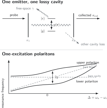
A cavity concentrates the vacuum field at an emitter, while its ports and parasitic losses set the total rate $\kappa$. The emitter also radiates into noncavity modes at rate $\gamma$. In the ideal one-excitation spectrum, the bare atom and cavity resonances hybridize and open a gap $2g$ at zero detuning. Loss broadens those polariton resonances and can hide the gap in a measured spectrum.

The mirrors in the figure are only one realization. Fabry–Pérot cavities, whispering-gallery resonators, photonic-crystal defects, microwave resonators, and nanophotonic cavities differ greatly in geometry but share the same local ingredients: a normalized mode field, an emitter transition, and specified decay channels.

Cavity Modes and the Vacuum Field

Resonance, linewidth, and quality factor

Let the selected cavity mode have angular frequency $\omega_c$ and annihilation operator $a$. Its total energy-decay rate is a sum over useful ports and unmonitored loss,

$$\kappa = \sum_j\kappa_j+\kappa_{\rm int}.$$

For an isolated Lorentzian resonance,

$$Q = \frac{\omega_c}{\kappa}.$$

A large $Q$ gives a long storage time; a small effective mode volume gives a large field per photon. Neither quantity by itself establishes strong coupling. A very high-$Q$ cavity can have poor spatial overlap with the emitter, and a tiny mode can be so lossy that coherent exchange is overdamped.

Normalized mode function

For a nondispersive dielectric and one nondegenerate mode, write the positive-frequency field as

$$\mathbf E^{(+)}(\mathbf r) = i \sqrt{\frac{\hbar\omega_c}{2\epsilon_0}}\, \mathbf f(\mathbf r)\,a,$$

with normalization

$$\int d^3r\, \epsilon_r(\mathbf r) \left|\mathbf f(\mathbf r)\right|^2 =1.$$

At a field antinode $\mathbf r_0$, an effective volume may be defined by

$$V_{\rm eff} = \frac{1}{ \epsilon_r(\mathbf r_0) \left|\mathbf f(\mathbf r_0)\right|^2 }.$$

For a dipole aligned with the local polarization, the corresponding maximum root-mean-square vacuum field is

$$E_{\rm vac,max} = \sqrt{ \frac{\hbar\omega_c}{ 2\epsilon_0\epsilon_r(\mathbf r_0)V_{\rm eff} } }.$$

This expression is a useful design estimate, not a universal definition for absorbing or strongly dispersive media. Quasinormal-mode normalization and the electromagnetic Green tensor are then safer tools. The conservative mode quantization is developed in Quantized Electromagnetic Modes.

What actually sets the overlap

The emitter samples the vector field at its position. The relevant overlap contains

• the standing-wave or traveling-wave amplitude at $\mathbf r_a$;
• alignment between the transition dipole and local polarization;
• angular-momentum and Clebsch–Gordan factors;
• the coherent superposition of Zeeman or hyperfine sublevels;
• averaging over motion, spectral diffusion, and technical drift.

Consequently, the maximum coupling quoted for a cavity geometry can be much larger than the time-averaged coupling in an experiment.

Atom–Field Coupling

In the electric-dipole approximation,

$$H_{\rm int} = -\mathbf d\mathbin{\cdot}\mathbf E(\mathbf r_a).$$

For transition dipole $\mathbf d_{eg}=\langle e|\mathbf d|g\rangle$, the rotating-wave single-photon coupling is

$$g(\mathbf r_a) = -i \sqrt{\frac{\omega_c}{2\hbar\epsilon_0}}\, \mathbf d_{eg}\mathbin{\cdot}\mathbf f(\mathbf r_a).$$

An overall phase of $g$ can be absorbed into $a$ or the atomic states for one emitter and one mode. Its magnitude is physical. At optimal position and orientation,

$$|g_{\rm max}| = \frac{d_{eg}E_{\rm vac,max}}{\hbar}.$$

The factor $g\sqrt{n+1}$ is the matrix element connecting $|e,n\rangle$ and $|g,n+1\rangle$. Even when the cavity begins in the vacuum, the $n=0$ matrix element remains $g$: the vacuum has zero mean electric field but nonzero field fluctuations.

After the rotating-wave approximation, the closed part of the minimal model is

$$\begin{aligned} \frac{H_{\rm JC}}{\hbar} ={}& \omega_c a^\dagger a + \omega_a\sigma_+\sigma_- \\ &+ g\,a\sigma_+ + g^*a^\dagger\sigma_-. \end{aligned}$$

This Hamiltonian is reliable when one transition and one mode are spectrally isolated, the coupling is weak compared with optical frequencies, and the mode function is not materially altered by the emitter. Ultrastrong coupling, dense multilevel structure, or overlapping resonances require a larger model.

Open-System Model and Rate Dictionary

A driven, lossy single-emitter model is

$$\begin{aligned} \dot\rho ={}& -\frac{i}{\hbar} \left[ H_{\rm JC}+H_{\rm drv}, \rho \right] + \kappa\mathcal D[a]\rho \\ &+ \gamma\mathcal D[\sigma_-]\rho + \frac{\gamma_\phi}{2} \mathcal D[\sigma_z]\rho, \end{aligned}$$

where

$$\mathcal D[L]\rho = L\rho L^\dagger - \frac12 \left\{ L^\dagger L,\rho \right\}.$$

With this normalization, pure dephasing contributes $\gamma_\phi$ to the optical coherence decay. The total transverse rate is

$$\gamma_\perp = \frac{\gamma}{2}+\gamma_\phi.$$

The model separates physically different quantities:

Symbol	Meaning	Decay or linewidth convention
$\kappa$	total cavity energy decay	cavity amplitude decays at $\kappa/2$
$\kappa_j$	coupling to port $j$	contributes to both damping and an output field
$\kappa_{\rm int}$	absorption, scattering, or other uncollected cavity loss	damps the mode without a useful port
$\gamma$	emitter population decay outside the modeled cavity channel	excited population decays at $\gamma$
$\gamma_\phi$	pure dephasing	adds directly to coherence decay
$\gamma_\perp$	total emitter coherence decay	optical amplitude decays at $\gamma_\perp$

When the emitter is weakly excited, set $\alpha=\langle a\rangle$ and $s=\langle\sigma_-\rangle$, approximate $\langle\sigma_z\rangle\simeq-1$, and drive port 1 with coherent amplitude $\beta_{\rm in}$. In a frame rotating at the probe frequency,

$$\begin{aligned} \dot\alpha ={}& \left( i\Delta_c-\frac{\kappa}{2} \right)\alpha -ig^*s -\sqrt{\kappa_1}\,\beta_{\rm in}, \\ \dot s ={}& \left( i\Delta_a-\gamma_\perp \right)s -ig\alpha, \end{aligned}$$

where $\Delta_c=\omega_{\rm p}-\omega_c$ and $\Delta_a=\omega_{\rm p}-\omega_a$. These are the equations of two damped coupled oscillators. They accurately describe weak-probe spectra, but they discard saturation and therefore cannot reproduce all single-photon nonlinearities or higher excitation manifolds.

Weak and Strong Coupling

Cooperativity

If pure dephasing is negligible, a standard single-emitter cooperativity is

$$C = \frac{4|g|^2}{\kappa\gamma}.$$

The numerator is the resonant emission rate $4|g|^2/\kappa$ into a broad cavity, and the denominator compares that rate with emission into other modes. With pure dephasing present, the weak-probe response is more directly organized by

$$C_\perp = \frac{2|g|^2}{\kappa\gamma_\perp}.$$

Since $\gamma_\perp=\gamma/2$ when $\gamma_\phi=0$, the two definitions then agree. A paper that instead calls the cavity field-amplitude decay rate $\kappa$ or calls the atomic half width $\gamma$ will display different factors of two or four. The invariant procedure is to reconstruct the equations of motion and identify which amplitudes or populations each rate damps.

High cooperativity means that the selected cavity channel competes successfully with unwanted emitter decoherence. It does not by itself mean that a photon oscillates coherently between atom and cavity. For example, a bad cavity can have

$$\kappa\gg |g|\gg\gamma \qquad\text{and}\qquad C\gg1.$$

It efficiently funnels emission into the cavity output while eliminating the intracavity field too quickly for several resolved swaps.

A practical regime map

• Perturbative weak coupling, $C_\perp\ll1$. The cavity weakly modifies an emitter, or the emitter weakly perturbs the cavity.
• Bad-cavity or Purcell regime, $\kappa\gg |g|,\gamma_\perp$. Eliminating the cavity gives enhanced irreversible emission into its output.
• High-cooperativity bad cavity, $C_\perp\gg1$ but $\kappa\gtrsim |g|$. Channeling and extinction can be strong without many coherent swaps.
• Strong coupling, $|g|$ above the relevant linewidth scales. Atom and cavity form resolvable hybrid modes and can exchange excitation coherently.
• Dispersive coupling, $|\Delta|\gg |g|\sqrt{n+1},\kappa,\gamma_\perp$. State-dependent frequency shifts dominate real exchange.
• Saturated response. Once the probe appreciably changes $\langle\sigma_z\rangle$, the linear coupled-oscillator formulas fail and nonlinear quantum dynamics matters.

These boundaries are crossovers, not phase transitions. A device can be strongly coupled for a stationary atom at an antinode but appear inhomogeneously broadened after averaging over motion. Conversely, a device without resolved normal-mode peaks may still have excellent cooperativity and single-emitter readout.

Vacuum Rabi Splitting

Ideal avoided crossing

In the one-excitation manifold of the lossless model, the two eigenfrequencies are

$$\omega_\pm = \frac{\omega_a+\omega_c}{2} \pm \frac12 \sqrt{\Delta^2+4|g|^2}.$$

Far from resonance, one branch is atom-like and the other cavity-like. Near $\Delta=0$, they hybridize into upper and lower polaritons. Their minimum frequency separation is

$$\omega_+-\omega_-=2|g|.$$

For an initial state $|e,0\rangle$ exactly on resonance and with no loss,

$$\begin{aligned} |\psi(t)\rangle ={}& \cos(gt)|e,0\rangle - i\sin(gt)|g,1\rangle, \\ P_e(t) ={}& \cos^2(gt). \end{aligned}$$

The first complete transfer occurs at $t=\pi/(2|g|)$, and the population oscillation has angular frequency $2|g|$. This time-domain exchange and the frequency-domain avoided crossing are two views of the same coupling.

Complex poles in a lossy system

In the weak-excitation sector, define the uncoupled complex frequencies

$$\widetilde\omega_c = \omega_c-\frac{i\kappa}{2}, \qquad \widetilde\omega_a = \omega_a-i\gamma_\perp.$$

The coupled poles are

$$\widetilde\omega_\pm = \frac{ \widetilde\omega_c+\widetilde\omega_a }{2} \pm \sqrt{ |g|^2 + \frac{ \left( \widetilde\omega_c-\widetilde\omega_a \right)^2 }{4} }.$$

On exact resonance and with $\gamma_\phi=0$, this reduces to

$$\widetilde\omega_\pm = \omega_0 - \frac{i(\kappa+\gamma)}{4} \pm \sqrt{ |g|^2 - \frac{(\kappa-\gamma)^2}{16} }.$$

The real parts separate once $|g|>|\kappa-\gamma|/4$. That algebraic condition is not a universal criterion for observing two peaks. If the common linewidth is broader than the separation, the peaks merge. Interference with a prompt reflected field can create a dip or asymmetry, and transmission, reflection, fluorescence, and intracavity spectra weight the poles differently.

Thus three statements should be kept distinct:

1. The closed Hamiltonian has an avoided crossing for every nonzero $g$.
2. The open linear response has two complex poles under a weaker, convention-dependent condition.
3. A particular experiment resolves two spectral features only when their separation, widths, port geometry, signal-to-noise ratio, and background permit it.

The conservative statement $|g|\gg\kappa,\gamma$ identifies an unambiguous strong-coupling limit, but many useful experiments operate near its boundary.

What makes the splitting quantum?

Two classical damped oscillators also exhibit normal-mode splitting. A spectral doublet alone therefore demonstrates coherent mode hybridization, not by itself the quantization of the electromagnetic field. The vacuum Rabi interpretation additionally relies on calibrated coupling to a single or known small number of emitters, operation near the zero-photon limit, and consistency with the one-quantum matrix element $g$. More distinctively quantum signatures include excitation-number-dependent $\sqrt{n+1}$ splittings, photon blockade, sub-Poissonian output, and conditional single-quantum dynamics.

Purcell Effect and Emission Channeling

Eliminating a broad cavity

Suppose the cavity is broader than the coherent coupling and changes much faster than the emitter. Adiabatic elimination gives an additional emitter-population decay rate into the cavity channel,

$$\Gamma_{\rm cav}(\Delta) = \frac{ |g|^2\kappa }{ \Delta^2+(\kappa/2)^2 }.$$

On resonance,

$$\Gamma_{\rm cav}(0) = \frac{4|g|^2}{\kappa}.$$

If $\gamma$ is the background radiative rate and nonradiative decay is negligible, then

$$\frac{\Gamma_{\rm cav}(0)}{\gamma} = C.$$

This is the weak-coupling meaning of cooperativity. The cavity has converted reversible coupling $g$ into an effectively irreversible decay channel because a cavity photon escapes on the short time scale $\kappa^{-1}$.

For an ideal dipole at the antinode of a weak-coupling dielectric cavity, the same result is often expressed as

$$F_P = \frac{3}{4\pi^2} \left( \frac{\lambda}{n} \right)^3 \frac{Q}{V_{\rm eff}},$$

multiplied in practice by spatial, polarization, and spectral-overlap factors. The Spontaneous Emission page develops the more general environmental and Green-tensor viewpoint.

Branching ratio is not collection efficiency

Let $\gamma_{\rm bg}$ denote residual radiative decay outside the selected cavity mode and $\gamma_{\rm nr}$ nonradiative loss. The probability that an excitation leaves through the cavity channel is

$$\beta_{\rm cav} = \frac{ \Gamma_{\rm cav} }{ \Gamma_{\rm cav} + \gamma_{\rm bg} + \gamma_{\rm nr} }.$$

Only a fraction $\kappa_{\rm col}/\kappa$ of those cavity photons leave by the desired port. Including propagation and detector efficiencies,

$$\eta_{\rm click} = \beta_{\rm cav} \frac{\kappa_{\rm col}}{\kappa} \eta_{\rm prop} \eta_{\rm det}.$$

A large Purcell factor can therefore coexist with poor detected efficiency if absorption dominates the cavity linewidth, the output is split among several ports, or the external optics have poor mode matching. Conversely, improving outcoupling can lower $Q$ and hence change the Purcell rate. Cavity design is an optimization over both emission and extraction.

Limits of the simple Purcell formula

The Lorentzian expression assumes weak excitation, one broad cavity mode, Markovian reservoirs, and an emitter narrower than or compatible with the cavity response. It must be reconsidered when

• coherent exchange is resolved;
• pure dephasing or spectral diffusion broadens the emitter;
• several cavity modes or transitions overlap;
• the cavity line is non-Lorentzian;
• nonradiative decay or blinking changes the emitter quantum yield;
• the electromagnetic environment is absorptive or strongly dispersive.

Purcell enhancement is thus a regime of cavity QED, not a synonym for strong coupling.

Cavity-Enhanced Measurement

Resonant extinction and transmission

The steady weak-probe cavity amplitude follows directly from the linear equations:

$$\alpha_{\rm ss} = - \frac{ \sqrt{\kappa_1}\,\beta_{\rm in} }{ \displaystyle \frac{\kappa}{2} -i\Delta_c + \frac{|g|^2}{ \gamma_\perp-i\Delta_a } }.$$

Together with the port relation

$$\beta_{{\rm out},j} = \beta_{{\rm in},j} + \sqrt{\kappa_j}\,\alpha_{\rm ss},$$

this predicts the coherent reflection or transmission signal in the sign convention used on the Input–Output Theory Overview. On double resonance, the emitter adds $|g|^2/\gamma_\perp$ to the cavity response denominator. Relative to an empty cavity, the intracavity field is reduced by a factor

$$\frac{1}{1+C_\perp}$$

for the same input and port convention. Even when individual fluorescence photons are hard to collect, this coherent perturbation can make one emitter visible in a bright transmitted or reflected probe.

The observed contrast is not a direct measurement of $C_\perp$ without a port model. Internal loss, mode mismatch, polarization leakage, prompt reflection, and detector normalization all affect the trace.

Dispersive readout

For a detuning large compared with the coupling across all occupied manifolds,

$$|\Delta| \gg |g|\sqrt{n+1}, \kappa, \gamma_\perp,$$

real excitation exchange is suppressed. To second order,

$$\begin{aligned} \frac{H_{\rm disp}}{\hbar} &\simeq \left( \omega_c+\chi\sigma_z \right)a^\dagger a \\ &\quad+ \frac{\omega_a+\chi}{2}\sigma_z, \\ \chi &= \frac{|g|^2}{\Delta}. \end{aligned}$$

The emitter state shifts the cavity resonance by opposite amounts, so a probe acquires a state-dependent amplitude or phase. Conversely, cavity photons shift the emitter and fluctuate in number, producing AC Stark shifts and measurement-induced dephasing. The scale

$$n_{\rm crit} \sim \frac{\Delta^2}{4|g|^2}$$

marks where the simplest dispersive expansion loses uniform validity; the exact threshold depends on the required accuracy and multilevel structure.

Dispersive does not mean backaction-free. Off-resonant photons can still scatter, and any record that distinguishes atomic states dephases their superposition when the record is ignored. A measurement is quantum nondemolition only with respect to a specified observable and effective Hamiltonian, over a specified time scale.

What the detector actually sees

Cavity-enhanced readout may use

• direct counting of cavity fluorescence or transmitted photons;
• extinction or transmission contrast of a coherent probe;
• homodyne phase shifts from a dispersive interaction;
• heterodyne records when both quadratures or an offset band are useful;
• correlations such as $g^{(2)}(\tau)$ to reveal nonlinear dynamics.

The receiver physics remains in Photon Counting and Homodyne and Heterodyne Detection. Conditional jumps, innovations, and trajectory backaction remain in the open-system cavity-QED map.

Several Emitters

For $N$ emitters in the weak-excitation sector, only one collective bright superposition couples to a single ideal cavity mode. Its coupling is

$$G = \sqrt{ \sum_{i=1}^{N}|g_i|^2 }.$$

For identical couplings, $G=\sqrt N\,|g|$. This enhancement follows from coherent addition of excitation amplitudes, not from $N$ independent emission rates. Dark collective states, inhomogeneous detunings, motion, and dipole-dipole interactions can invalidate the simple two-oscillator description. A measured $\sqrt N$ splitting therefore requires control or calibration of the participating ensemble.

Reading an Experiment

A defensible cavity-QED analysis can be organized as follows:

1. State the rate convention. Say whether $\kappa$ is an energy decay, field decay, half width, or full width, and do the same for $\gamma$.
2. Calibrate the empty cavity. Determine resonance frequency, loaded linewidth, external port rates, internal loss, and spatial mode.
3. Identify the emitter channel. Measure or justify its transition frequency, polarization, radiative rate, pure dephasing, and level structure.
4. Estimate the overlap. Separate the ideal $g_{\rm max}$ from reductions caused by position, orientation, motion, and internal-state preparation.
5. Fit complex amplitudes when possible. Power spectra discard phase and can confound a pole with an interference zero.
6. Test probe-power dependence. A weak-probe model should cease to fit as the emitter saturates; unexplained power dependence is a warning.
7. Compare independent observables. Ringdown constrains $\kappa$, lifetime data constrain $\gamma$, avoided crossings constrain $g$, and output correlations test nonlinear quantum behavior.
8. Report collection separately. Keep $\beta_{\rm cav}$, $\kappa_{\rm col}/\kappa$, propagation efficiency, and detector efficiency as distinct factors.

Computational Notebook

The Cavity QED Simulation Notebook provides reproducible dressed-spectrum, vacuum-Rabi, collapse–revival, photon-cutoff, and small Lindblad-loss benchmarks. Use this page for the physical rate dictionary and experiment-facing interpretation; use the notebook for finite-basis construction and numerical validation.

Common Mistakes

• Equating high $Q$ with strong coupling. The mode volume, dipole overlap, and emitter linewidth are equally important.
• Mixing linewidth conventions. Comparing a cavity full width with an atomic half width creates spurious factors of two.
• Calling every doublet vacuum Rabi splitting. Classical hybridization, multiple emitters, polarization modes, or prompt-path interference can also produce two features.
• Equating $C>1$ with resolved coherent swaps. High-cooperativity bad-cavity systems are common and useful.
• Using $g_{\rm max}$ as the measured coupling. Position, polarization, internal state, and motion reduce the realized value.
• Treating the Purcell factor as detected efficiency. Emission into a cavity, escape through the desired port, transmission, and detection are separate stages.
• Applying a weak-probe spectrum after saturation. Once $\langle\sigma_z\rangle$ changes appreciably, the linear oscillator equations no longer close.
• Calling dispersive readout backaction-free. Information extraction, photon-number fluctuations, and residual scattering all disturb the emitter.

Exercises

Exercise 1: Vacuum field and maximum coupling

An empty-space cavity mode has wavelength $\lambda=780\ \mathrm{nm}$ and effective volume

$$V_{\rm eff} = 1000\ \mu\mathrm m^3.$$

An optimally oriented transition has dipole magnitude $d_{eg}=3ea_0$. Estimate $E_{\rm vac,max}$ and $g_{\rm max}/(2\pi)$. Use $e=1.602\times10^{-19}\ \mathrm C$, $a_0=5.292\times10^{-11}\ \mathrm m$, and $c=2.998\times10^8\ \mathrm{m\,s^{-1}}$.

Solution

The angular frequency and mode volume in SI units are

$$\begin{gathered} \omega_c = \frac{2\pi c}{\lambda} , \\ \omega_c \simeq 2.414\times10^{15}\ \mathrm{s^{-1}}, \\ V_{\rm eff} = 1000\times10^{-18}\ \mathrm m^3 , \\ V_{\rm eff} = 1.00\times10^{-15}\ \mathrm m^3. \end{gathered}$$

For $n=1$,

$$\begin{aligned} E_{\rm vac,max} &= \sqrt{ \frac{\hbar\omega_c}{2\epsilon_0V_{\rm eff}} } \\ &\simeq 3.79\times10^3\ \mathrm{V\,m^{-1}}. \end{aligned}$$

The dipole magnitude is

$$d_{eg} = 3ea_0 \simeq 2.54\times10^{-29}\ \mathrm{C\,m}.$$

Therefore

$$\begin{aligned} g_{\rm max} &= \frac{d_{eg}E_{\rm vac,max}}{\hbar} \simeq 9.14\times10^8\ \mathrm{s^{-1}}, \\ \frac{g_{\rm max}}{2\pi} &\simeq 145\ \mathrm{MHz}. \end{aligned}$$

This is an ideal spatial and polarization value. The measured coupling will be smaller if the emitter is not at the antinode or if the transition dipole does not align with the local mode.

Exercise 2: Spatial, polarization, and internal-state overlap

An emitter in a standing-wave cavity has

$$g = g_{\rm max} \cos(kz) \cos\theta C_{\rm ang},$$

where $\theta$ is the angle between the dipole and local polarization and $C_{\rm ang}$ is an angular-momentum amplitude. Take $z=\lambda/8$ measured from an antinode, $\theta=60^\circ$, and $C_{\rm ang}=\sqrt{2/3}$.

1. Find $g/g_{\rm max}$.
2. Find $C/C_{\rm max}$ if all decay rates are unchanged.

Solution

Since $k=2\pi/\lambda$,

$$\cos(kz) = \cos\left(\frac{\pi}{4}\right) = \frac{1}{\sqrt2}.$$

The full amplitude ratio is

$$\begin{aligned} \frac{g}{g_{\rm max}} &= \frac{1}{\sqrt2} \left(\frac12\right) \sqrt{\frac23} \\ &= \frac{1}{2\sqrt3} \simeq 0.289. \end{aligned}$$

Cooperativity scales as $|g|^2$, so

$$\frac{C}{C_{\rm max}} = \left| \frac{g}{g_{\rm max}} \right|^2 = \frac1{12} \simeq 0.0833.$$

Three moderate amplitude-overlap reductions have lowered the cooperativity by a factor of twelve. This is why quoting only the geometric $g_{\rm max}$ can be misleading.

Exercise 3: High cooperativity without strong coupling

A cavity and emitter are resonant, with

$$\begin{gathered} \frac{g}{2\pi}=40\ \mathrm{MHz}, \\ \frac{\kappa}{2\pi}=400\ \mathrm{MHz}, \\ \frac{\gamma}{2\pi}=0.40\ \mathrm{MHz}, \end{gathered}$$

and negligible pure dephasing.

1. Calculate the cooperativity.
2. Calculate the resonant bad-cavity emission rate $\Gamma_{\rm cav}/(2\pi)$.
3. Classify the system.

Solution

All three quoted numbers use the same angular-frequency conversion, so the factors of $2\pi$ cancel in ratios:

$$C = \frac{ 4(40)^2 }{ (400)(0.40) } = 40.$$

The eliminated-cavity rate is

$$\frac{\Gamma_{\rm cav}}{2\pi} = \frac{ 4(40\ \mathrm{MHz})^2 }{ 400\ \mathrm{MHz} } = 16\ \mathrm{MHz}.$$

Thus cavity-mediated emission is forty times faster than background emission. Nevertheless,

$$\kappa=10g,$$

so a cavity excitation escapes much faster than one coherent atom-cavity swap. This is a high-cooperativity bad-cavity system, not an unambiguous resolved-strong-coupling system.

Exercise 4: Dissipative polariton poles

On exact resonance, a system with negligible pure dephasing has

$$\begin{gathered} \frac{g}{2\pi}=10\ \mathrm{MHz}, \\ \frac{\kappa}{2\pi}=8\ \mathrm{MHz}, \\ \frac{\gamma}{2\pi}=2\ \mathrm{MHz}. \end{gathered}$$

Find the real-frequency separation of the two weak-excitation poles and the power linewidth associated with their common imaginary part. Would a doublet be expected in a clean spectrum?

Solution

Writing every rate after division by $2\pi$ in megahertz, the real offset of each pole is

$$\begin{aligned} \frac{\Omega_{\rm pole}}{2\pi} &= \sqrt{ (10)^2 - \frac{(8-2)^2}{16} } \ \mathrm{MHz} \\ &= \sqrt{97.75}\ \mathrm{MHz} \simeq 9.89\ \mathrm{MHz}. \end{aligned}$$

The pole separation is therefore

$$\frac{ \operatorname{Re} \left( \widetilde\omega_+ - \widetilde\omega_- \right) }{2\pi} \simeq 19.8\ \mathrm{MHz}.$$

The common imaginary part has magnitude

$$\frac{\kappa+\gamma}{4(2\pi)} = 2.5\ \mathrm{MHz}.$$

An amplitude pole with imaginary part $-2\pi(2.5\ \mathrm{MHz})$ produces a Lorentzian power full width of approximately $5.0\ \mathrm{MHz}$. The separation is nearly four times that width, so a clean, well-coupled measurement channel should resolve two features. Interference backgrounds or inhomogeneous broadening could still obscure them.

Exercise 5: Purcell channeling and click probability

A weakly coupled emitter has

$$\begin{gathered} \frac{g}{2\pi}=25\ \mathrm{MHz}, \\ \frac{\kappa}{2\pi}=250\ \mathrm{MHz}, \\ \frac{\Delta}{2\pi}=125\ \mathrm{MHz}. \end{gathered}$$

Its noncavity rates are $\gamma_{\rm bg}/(2\pi)=1.0\ \mathrm{MHz}$ and $\gamma_{\rm nr}/(2\pi)=0.5\ \mathrm{MHz}$. The useful port has $\kappa_{\rm col}/\kappa=0.70$, while $\eta_{\rm prop}=0.80$ and $\eta_{\rm det}=0.60$.

1. Find $\Gamma_{\rm cav}/(2\pi)$ and $\beta_{\rm cav}$.
2. Find the probability that one initial emitter excitation produces a detector click through the selected path.

Solution

Using the common megahertz units,

$$\begin{aligned} \frac{\Gamma_{\rm cav}}{2\pi} &= \frac{ (25)^2(250) }{ (125)^2+(250/2)^2 } \ \mathrm{MHz} \\ &= 5.0\ \mathrm{MHz}. \end{aligned}$$

The cavity branching ratio is

$$\beta_{\rm cav} = \frac{5.0}{5.0+1.0+0.5} \simeq 0.769.$$

The total click probability is

$$\begin{aligned} \eta_{\rm click} &= (0.769)(0.70)(0.80)(0.60) \\ &\simeq 0.258. \end{aligned}$$

About $77\%$ of excitations enter the cavity channel, but only about $26\%$ produce a registered click. Conflating those two numbers would overstate the system efficiency by almost a factor of three.

Exercise 6: Adiabatic elimination

In a frame rotating at the emitter frequency, let the no-jump single-excitation amplitudes obey

$$\begin{aligned} \dot c_e &= -igc_c, \\ \dot c_c &= \left( i\Delta-\frac{\kappa}{2} \right)c_c -ig^*c_e. \end{aligned}$$

Assume $\kappa$ and $|\Delta|$ are large enough that $\dot c_c\simeq0$. Eliminate $c_c$ and identify the cavity-induced population-decay rate and frequency shift.

Solution

Setting the fast derivative to zero gives

$$c_c \simeq - \frac{ig^*}{ \kappa/2-i\Delta } c_e.$$

Substitution into the emitter equation yields

$$\begin{aligned} \dot c_e &= - \frac{|g|^2}{ \kappa/2-i\Delta } c_e \\ &= - \frac{ |g|^2\kappa/2 }{ \Delta^2+(\kappa/2)^2 } c_e \\ &\quad -i \frac{ |g|^2\Delta }{ \Delta^2+(\kappa/2)^2 } c_e. \end{aligned}$$

Writing

$$\dot c_e = - \left( \frac{\Gamma_{\rm cav}}{2} +i\delta_{\rm cav} \right)c_e,$$

we identify

$$\begin{gathered} \Gamma_{\rm cav} = \frac{ |g|^2\kappa }{ \Delta^2+(\kappa/2)^2 }, \\ \delta_{\rm cav} = \frac{ |g|^2\Delta }{ \Delta^2+(\kappa/2)^2 }. \end{gathered}$$

The same eliminated susceptibility produces a dissipative rate from its real part and a reactive frequency shift from its imaginary part. Reversing the definition of detuning reverses the sign of $\delta_{\rm cav}$ but not the decay rate.

Exercise 7: Dispersive scale and critical photon number

An atom-cavity system has

$$\begin{gathered} \frac{g}{2\pi}=20\ \mathrm{MHz}, \\ \frac{\Delta}{2\pi}=1.00\ \mathrm{GHz}, \\ \frac{\kappa}{2\pi}=2.0\ \mathrm{MHz}. \end{gathered}$$

1. Estimate $\chi/(2\pi)$ and $n_{\rm crit}$.
2. For $\bar n=25$, evaluate $g\sqrt{\bar n+1}/|\Delta|$.
3. Compare the separation between the two state-dependent cavity frequencies with the empty-cavity linewidth.

Solution

The dispersive shift is

$$\frac{\chi}{2\pi} = \frac{ (20\ \mathrm{MHz})^2 }{ 1000\ \mathrm{MHz} } = 0.40\ \mathrm{MHz}.$$

The conventional critical scale is

$$n_{\rm crit} \sim \frac{(1000)^2}{4(20)^2} = 625.$$

At $\bar n=25$,

$$\frac{ g\sqrt{\bar n+1} }{ |\Delta| } = \frac{ 20\sqrt{26} }{ 1000 } \simeq 0.102.$$

The leading dispersive expansion is plausible, with corrections controlled by a parameter of order $10^{-2}$ in quantities that begin at second order, though precision work should retain higher orders.

The two atomic states shift the cavity by $\pm\chi$, so their resonance separation is

$$\frac{2\chi}{2\pi} = 0.80\ \mathrm{MHz}.$$

This is smaller than the $2.0\ \mathrm{MHz}$ cavity full width. The states need not produce two resolved peaks: a phase-sensitive measurement can still distinguish their different complex transmission amplitudes after sufficient integration.

Exercise 8: Collective bright-state coupling

Twenty-five identical emitters couple with equal phase and $g/(2\pi)=3.0\ \mathrm{MHz}$ to one cavity mode. Take

$$\frac{\kappa}{2\pi}=20\ \mathrm{MHz}, \qquad \frac{\gamma}{2\pi}=1.0\ \mathrm{MHz},$$

with no pure dephasing or inhomogeneous broadening.

1. Find $G/(2\pi)$ and the collective cooperativity.
2. Estimate the resonant separation of the two collective weak-excitation poles.
3. Explain why the result need not survive arbitrary emitter detunings.

Solution

For equal couplings,

$$\frac{G}{2\pi} = \sqrt{25} \left( 3.0\ \mathrm{MHz} \right) = 15\ \mathrm{MHz}.$$

The collective cooperativity is

$$C_N = \frac{4G^2}{\kappa\gamma} = \frac{4(15)^2}{(20)(1)} = 45.$$

The pole separation follows from the single-bright-mode formula:

$$\begin{aligned} \frac{\Delta\omega_{\rm poles}}{2\pi} &= 2 \sqrt{ (15)^2 - \frac{(20-1)^2}{16} } \ \mathrm{MHz} \\ &\simeq 28.5\ \mathrm{MHz}. \end{aligned}$$

Identical resonance frequencies make one collective superposition bright and leave orthogonal superpositions dark. Inhomogeneous detunings mix those collective states and dephase their amplitudes. If the detuning spread is comparable with $G$ or the polariton linewidths, the simple $\sqrt N$ doublet broadens or fragments.

References

1. E. M. Purcell, “Spontaneous emission probabilities at radio frequencies,” Physical Review 69, 681 (1946).
2. E. T. Jaynes and F. W. Cummings, “Comparison of quantum and semiclassical radiation theories with application to the beam maser,” Proceedings of the IEEE 51, 89–109 (1963).
3. G. Rempe, H. Walther, and N. Klein, “Observation of quantum collapse and revival in a one-atom maser,” Physical Review Letters 58, 353–356 (1987).
4. R. J. Thompson, G. Rempe, and H. J. Kimble, “Observation of normal-mode splitting for an atom in an optical cavity,” Physical Review Letters 68, 1132–1135 (1992).
5. M. Brune, F. Schmidt-Kaler, A. Maali, J. Dreyer, E. Hagley, J. M. Raimond, and S. Haroche, “Quantum Rabi oscillation: A direct test of field quantization in a cavity,” Physical Review Letters 76, 1800–1803 (1996).
6. C. J. Hood, M. S. Chapman, T. W. Lynn, and H. J. Kimble, “Real-time cavity QED with single atoms,” Physical Review Letters 80, 4157–4160 (1998).
7. J. M. Raimond, M. Brune, and S. Haroche, “Manipulating quantum entanglement with atoms and photons in a cavity,” Reviews of Modern Physics 73, 565–582 (2001).
8. H. Mabuchi and A. C. Doherty, “Cavity quantum electrodynamics: Coherence in context,” Science 298, 1372–1377 (2002).
9. J. P. Reithmaier et al., “Strong coupling in a single quantum dot–semiconductor microcavity system,” Nature 432, 197–200 (2004).
10. A. Wallraff et al., “Strong coupling of a single photon to a superconducting qubit using circuit quantum electrodynamics,” Nature 431, 162–167 (2004).
11. K. J. Vahala, “Optical microcavities,” Nature 424, 839–846 (2003).
12. H. Walther, B. T. H. Varcoe, B.-G. Englert, and T. Becker, “Cavity quantum electrodynamics,” Reports on Progress in Physics 69, 1325–1382 (2006).
13. S. Haroche and J.-M. Raimond, Exploring the Quantum: Atoms, Cavities, and Photons (Oxford University Press, 2006).
14. H. J. Carmichael, Statistical Methods in Quantum Optics 2: Non-Classical Fields (Springer, 2008).
15. D. F. Walls and G. J. Milburn, Quantum Optics, 2nd ed. (Springer, 2008).
16. A. Reiserer and G. Rempe, “Cavity-based quantum networks with single atoms and optical photons,” Reviews of Modern Physics 87, 1379–1418 (2015).
17. P. Lodahl, S. Mahmoodian, and S. Stobbe, “Interfacing single photons and single quantum dots with photonic nanostructures,” Reviews of Modern Physics 87, 347–400 (2015).
18. J. M. Gérard, “Solid-state cavity-quantum electrodynamics with self-assembled quantum dots,” in Single Quantum Dots: Fundamentals, Applications and New Concepts, Topics in Applied Physics 90, 269–314 (Springer, 2003).

Frontier Context

Cavity and Circuit QED Frontiers tracks dated evidence and open questions in ultrastrong and multimode coupling, waveguide QED, superconducting circuits, hybrid transducers, and bosonic quantum memories. The definitions and single-mode derivations remain canonical on this page.