Correlation Functions

Optical coherence is not one number and not a synonym for narrow linewidth. It is a hierarchy of correlation functions that predicts how field samples at different positions, times, polarizations, and detector channels interfere or produce joint photoevents. First-order coherence controls amplitude interference. Second-order coherence controls ideal coincidence statistics. Higher orders control increasingly detailed multiphoton records.

The hierarchy is operational. In Glauber photodetection theory, an absorbing detector selects a positive-frequency field operator at each event, and an $n$-fold coincidence samples a normally ordered $2n$-operator expectation value. The ordering is part of the physics, not decorative notation. Symmetrized noise, time-ordered Green functions, and retarded response functions answer different questions.

A trustworthy correlation statement identifies:

• every space-time, polarization, and mode argument;
• the operator ordering and state;
• whether the field is stationary, pulsed, or explicitly time dependent;
• normalization and treatment of zero intensity;
• filtering, finite gates, loss, background, and detector timing response;
• whether the result is raw, corrected, inferred, or model predicted.

Without these declarations, a value such as $g^{(2)}(0)=1$ does not identify a state or even a unique experiment.

Canonical Scope

This page is the canonical home for optical coherence functions:

• the first-order kernel $G^{(1)}$ and degree of coherence $g^{(1)}$;
• the second-order photodetection function $G^{(2)}$ and normalized coincidence function $g^{(2)}$;
• the general normally ordered Glauber hierarchy;
• coherent, thermal, and number-state examples;
• the relation between gated count factorial moments and continuous-time correlations;
• classical Cauchy–Schwarz bounds and sufficient nonclassicality tests;
• stationarity, spectral coherence, multimode averaging, filtering, and detector convolution.

Photon Counting owns the calibrated detector response, efficiency, dark counts, dead time, and response matrices. Hanbury Brown–Twiss Interferometry owns the detailed intensity-interferometer geometry and data normalization, while Photon Antibunching owns the single-emitter signature and its experimental pitfalls. Coherent Light, Thermal Light, and Photon Number States own those source states.

Generic connected, retarded, many-body, and spectral correlators belong to Correlation Functions Overview. Environmental memory, KMS relations, and bath ordering belong to Bath Correlation Functions.

Field and Detector Notation

Detection coordinate

Write

$$x=(\mathbf r,t,\lambda),$$

where $\lambda$ abbreviates polarization, detector channel, spectral filter, or other resolved labels. Let

$$\hat E^{(+)}(x)$$

be the scalar positive-frequency field after projection onto the detector response. Its adjoint is

$$\hat E^{(-)}(x) = \left[ \hat E^{(+)}(x) \right]^\dagger.$$

Vector fields require polarization contractions or a coherence matrix. The scalar notation below assumes that those choices have already been made.

Constants containing detector responsivity can be restored when absolute rates are needed. Correlation ratios often cancel a common constant, but they do not cancel mode mismatch or channel-dependent response automatically.

Intensity notation

The normally ordered optical intensity operator at $x$ is proportional to

$$\hat I(x) = \hat E^{(-)}(x)\hat E^{(+)}(x).$$

Its expectation,

$$I(x) = \left\langle\hat I(x)\right\rangle,$$

sets the ideal first-order absorption rate. The symbol $I$ below denotes this normally ordered mean unless stated otherwise.

Vacuum has a nonzero symmetrized field variance but

$$\langle0| \hat E^{(-)}(x)\hat E^{(+)}(x) |0\rangle = 0$$

in an ideal empty mode. This is one reason ordering conventions cannot be interchanged casually.

First-Order Coherence

Mutual coherence function

The first-order optical correlation is

$$G^{(1)}(x_1,x_2) = \left\langle \hat E^{(-)}(x_1) \hat E^{(+)}(x_2) \right\rangle.$$

Its diagonal is the mean intensity:

$$G^{(1)}(x,x)=I(x).$$

The kernel is Hermitian,

$$G^{(1)}(x_2,x_1) = \left[ G^{(1)}(x_1,x_2) \right]^*,$$

and positive semidefinite. For arbitrary complex coefficients $c_j$,

$$\sum_{j,k} c_j^*c_k G^{(1)}(x_j,x_k) \ge0.$$

This follows because the left side is

$$\left\langle \hat A^\dagger\hat A \right\rangle, \qquad \hat A = \sum_k c_k\hat E^{(+)}(x_k).$$

Normalized degree of coherence

When both local intensities are nonzero, define

$$g^{(1)}(x_1,x_2) = \frac{ G^{(1)}(x_1,x_2) }{ \sqrt{I(x_1)I(x_2)} }.$$

The Cauchy–Schwarz inequality gives

$$\left| g^{(1)}(x_1,x_2) \right| \le1.$$

The magnitude measures normalized amplitude coherence between the two samples; the argument gives their correlation phase. If either intensity vanishes, the normalized ratio is undefined even though the unnormalized kernel is well defined.

Interference visibility

Suppose two sampled fields are recombined with a controllable phase $\phi$. After absorbing fixed transmission factors into $I_1$ and $I_2$, the mean output intensity is

$$\begin{aligned} I(\phi) ={}& I_1+I_2 \\ &+ 2\sqrt{I_1I_2}\, \operatorname{Re} \left[ e^{i\phi}g_{12}^{(1)} \right]. \end{aligned}$$

The fringe visibility

$$\mathcal V \equiv \frac{I_{\max}-I_{\min}} {I_{\max}+I_{\min}}$$

is therefore

$$\mathcal V = \frac{ 2\sqrt{I_1I_2} }{ I_1+I_2 } \left|g_{12}^{(1)}\right|.$$

For balanced intensities,

$$\mathcal V = \left|g_{12}^{(1)}\right|.$$

Unequal intensity lowers visibility even for perfect mutual coherence. Conversely, high visibility establishes first-order coherence for the selected samples but does not establish Poisson statistics or a coherent quantum state.

Coherence matrix

For several polarization or spatial components, define

$$\Gamma_{\mu\nu}^{(1)}(x_1,x_2) = \left\langle \hat E_\mu^{(-)}(x_1) \hat E_\nu^{(+)}(x_2) \right\rangle.$$

This matrix carries intensity, polarization, and mutual coherence together. Tracing over unresolved components can reduce measured visibility. A scalar $g^{(1)}$ is meaningful only after specifying the projections or contractions used by the optical system and detector.

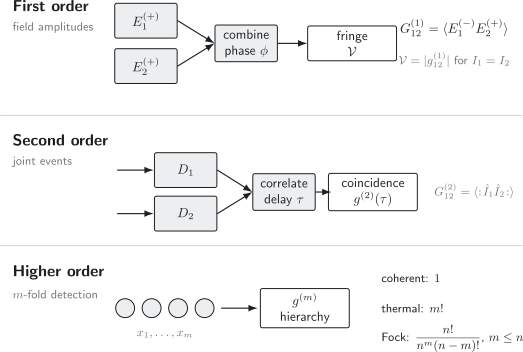
The optical hierarchy associates order one with field-amplitude interference, order two with joint intensity events, and order $m$ with $m$-fold photodetection. The familiar equal-mode values $1$, $m!$, and $n!/[n^m(n-m)!]$ summarize different states but do not replace the full space-time functions; the number-state expression applies for $m\leq n$ and vanishes for $m>n$.

Stationarity and Spectrum

Time-translation invariance

For a stationary field,

$$G^{(1)}(t_1,t_2) = G^{(1)}(t_2-t_1).$$

With the convention

$$G^{(1)}(\tau) = \left\langle \hat E^{(-)}(t) \hat E^{(+)}(t+\tau) \right\rangle,$$

stationarity implies

$$G^{(1)}(-\tau) = \left[ G^{(1)}(\tau) \right]^*.$$

Stationarity is an ensemble property. A finite record can drift, blink, age, or mix several operating points even when a time-averaged plot appears smooth.

Wiener–Khinchin relation

Choose the spectral convention

$$S(\omega) = \frac1{2\pi} \int_{-\infty}^{\infty} d\tau\, e^{i\omega\tau} G^{(1)}(\tau).$$

Then

$$G^{(1)}(\tau) = \int_{-\infty}^{\infty} d\omega\, e^{-i\omega\tau}S(\omega).$$

For a stationary physical field, $S(\omega)$ is nonnegative in the relevant analytic-signal convention. The spectral width and temporal decay of $g^{(1)}$ are Fourier related, but “coherence time” has several definitions.

A common integral convention is

$$\tau_c = \int_{-\infty}^{\infty} d\tau\, \left|g^{(1)}(\tau)\right|^2.$$

Other conventions use a $1/e$ width, half width at half maximum, or integral of $|g^{(1)}|$. Numerical coherence times should therefore be accompanied by their definition. Linewidth and Coherence applies these alternatives to laser phase diffusion, frequency-noise PSDs, and measured cw line shapes.

Two line-shape examples

For a Lorentzian spectrum centered at $\omega_0$ with field-correlation decay rate $\gamma$,

$$g^{(1)}(\tau) = e^{-i\omega_0\tau} e^{-\gamma|\tau|}.$$

For a Gaussian spectrum with rms width $\sigma_\omega$,

$$g^{(1)}(\tau) = e^{-i\omega_0\tau} e^{-\sigma_\omega^2\tau^2/2}.$$

The oscillatory carrier and decaying envelope contain different information. Removing a carrier in a rotating frame does not lengthen the physical coherence envelope.

Second-Order Coherence

Joint photodetection function

The normally ordered second-order function is

$$\begin{aligned} G^{(2)}(x_1,x_2) ={}& \bigl\langle \hat E^{(-)}(x_1) \hat E^{(-)}(x_2) \\ &\quad\times \hat E^{(+)}(x_2) \hat E^{(+)}(x_1) \bigr\rangle. \end{aligned}$$

It is nonnegative because it has the form

$$G^{(2)}(x_1,x_2) = \left\langle \hat A^\dagger\hat A \right\rangle,$$

with

$$\hat A = \hat E^{(+)}(x_2) \hat E^{(+)}(x_1).$$

For ideal weak absorbers, $G^{(2)}$ is proportional to the joint density for two photoevents at the declared coordinates. Detector response and finite gates turn this density into integrated probabilities.

Normalized second-order coherence

When $I(x_1)I(x_2)\ne0$, define

$$g^{(2)}(x_1,x_2) = \frac{ G^{(2)}(x_1,x_2) }{ I(x_1)I(x_2) }.$$

For one stationary channel,

$$g^{(2)}(\tau) = \frac{G^{(2)}(\tau)}{I^2},$$

where

$$\begin{aligned} G^{(2)}(\tau) ={}& \bigl\langle \hat E^{(-)}(t) \hat E^{(-)}(t+\tau) \\ &\quad\times \hat E^{(+)}(t+\tau) \hat E^{(+)}(t) \bigr\rangle. \end{aligned}$$

At large delays, independent stationary samples often give

$$g^{(2)}(\tau)\longrightarrow1,$$

but this limit can fail for nonergodic mixtures, blinking, periodic driving, long memory, or conditioning.

Conditional-rate interpretation

For a stationary ideal point process with mean detection rate $\bar R$,

$$\bar R\,g^{(2)}(\tau)$$

is the conditional event rate at delay $\tau$ given an event at the origin, under the standard weak-detection assumptions. Thus:

• $g^{(2)}(\tau)>1$ means enhanced conditional detection;
• $g^{(2)}(\tau)<1$ means suppressed conditional detection;
• $g^{(2)}(\tau)=1$ means no second-order excess at that delay.

This interpretation concerns events in the selected channel. It does not imply a force between photons, a literal packet size, or a complete description of the field state.

Normal ordering and shot noise

At one point,

$$G^{(2)}(x,x) = \left\langle : \hat I(x)^2 : \right\rangle,$$

not the unordered $\langle\hat I^2\rangle$. For one mode,

$$\hat a^\dagger\hat a^\dagger\hat a\hat a = \hat N(\hat N-1).$$

The falling factorial excludes pairing one registered event with itself. When ordinary count variance is reconstructed, the missing diagonal returns as the Poisson shot-noise term.

Pulsed and Gated Correlations

One selected pulse mode

For a pulse described by one selected mode with number operator $\hat N$, the zero-delay pulsed quantity is

$$g_{\mathrm p}^{(2)}[0] = \frac{ \langle\hat N(\hat N-1)\rangle }{ \langle\hat N\rangle^2 }.$$

Square brackets emphasize a discrete pulse lag. This quantity is not automatically the same as an infinitesimal continuous-time $g^{(2)}(0)$. It integrates all temporal structure accepted within the pulse and detection gate.

Factorial moments in a gate

Let $N_G$ be the ideal count in a gate $G$. Under linear photodetection,

$$\begin{aligned} \left\langle (N_G)_m \right\rangle ={}& \int_G dx_1\cdots \int_G dx_m \\ &\times G^{(m)}(x_1,\ldots,x_m), \end{aligned}$$

up to the declared responsivity factors. Here

$$(N_G)_m = N_G(N_G-1)\cdots(N_G-m+1).$$

Changing the gate changes the measured mode mixture and therefore can change the normalized correlation even when the source is unchanged.

Count variance from temporal coherence

For one stationary stream with mean ideal rate $\bar R$ and a gate of duration $T$,

$$\langle N_T\rangle = \bar R T.$$

The general factorial second moment is

$$\begin{aligned} \langle N_T(N_T-1)\rangle ={}& \bar R^2 \int_0^Tdt \int_0^Tdt' \\ &\times g^{(2)}(t'-t). \end{aligned}$$

When the same-channel stationary correlation is even in delay,

$$\mathcal C_T := \int_0^T d\tau\, (T-\tau) \left[ g^{(2)}(\tau)-1 \right].$$

The count variance is then

$$\operatorname{Var}(N_T) = \bar R T + 2\bar R^2\mathcal C_T.$$

The first term is shot noise. Positive integrated excess produces super-Poissonian count variance; negative integrated excess can produce sub-Poissonian variance. A local dip at zero delay does not by itself fix the long-gate Fano factor because the complete correlation area matters.

Higher-Order Glauber Correlations

Detection-diagonal hierarchy

For $m$ detection coordinates, define the ordered absorption product

$$\hat A_m(\mathbf x) := \hat E^{(+)}(x_m)\cdots \hat E^{(+)}(x_1),$$

where $\mathbf x=(x_1,\ldots,x_m)$. The detection-diagonal correlation is

$$G^{(m)}(\mathbf x) := \left\langle \hat A_m^\dagger(\mathbf x) \hat A_m(\mathbf x) \right\rangle \geq 0.$$

Expanding $\hat A_m^\dagger\hat A_m$ reverses the positive-frequency factors relative to the negative-frequency factors. The positive-operator form also makes the nonnegativity of an ideal joint photodetection rate explicit.

The normalized detection-diagonal function is

$$g^{(m)}(x_1,\ldots,x_m) = \frac{ G^{(m)}(x_1,\ldots,x_m) }{ \prod_{j=1}^{m}I(x_j) },$$

when every denominator is nonzero.

Full two-set kernel

The more general coherence kernel keeps separate negative- and positive-frequency coordinates:

$$G^{(m)}(\mathbf x;\mathbf y) := \left\langle \hat A_m^\dagger(\mathbf x) \hat A_m(\mathbf y) \right\rangle.$$

Here $\mathbf y=(y_1,\ldots,y_m)$. Expanding the compact notation gives negative-frequency factors at $\mathbf x$ followed by the reversed positive-frequency factors at $\mathbf y$. The detection-diagonal function sets $y_j=x_j$. Keeping the full kernel is important in coherence theory, propagation, and interferometric transformations.

Coherence order

A field is first-order coherent over a domain when its first-order kernel factorizes there:

$$G^{(1)}(x,y) = \mathcal E^*(x)\mathcal E(y).$$

Full Glauber coherence requires factorization of the entire normally ordered hierarchy:

$$\begin{aligned} G^{(m)}(\mathbf x;\mathbf y) ={}& \prod_{j=1}^{m} \mathcal E^*(x_j) \\ &\times \prod_{j=1}^{m} \mathcal E(y_j) \end{aligned}$$

for all relevant orders and coordinates. An ideal multimode coherent state satisfies this condition. Demonstrating one value such as $g^{(2)}(0)=1$ does not demonstrate full coherence.

Correlation hierarchy is not always state tomography

Photodetection correlations are invariant under a global optical phase. A coherent state with unknown uniformly distributed global phase can reproduce the same phase-insensitive normally ordered number correlations as a fixed coherent amplitude. Low-order correlation data also leave many distinct states compatible with the observations.

The complete state requires an informationally complete measurement, often using a phase reference. Phase-Space Distributions and homodyne tomography address that larger reconstruction problem.

Standard State Examples

Coherent light

For a coherent state, each positive-frequency field annihilation operator acts by its classical complex amplitude. Therefore all normally ordered correlations factorize. Wherever the intensity is nonzero,

$$g_{\mathrm{coh}}^{(m)} = 1.$$

The result holds across coordinates for an ideal coherent field after deterministic linear propagation. Technical amplitude or phase fluctuations can produce a mixture whose measured coherence is lower or whose intensity correlations differ from one.

One-mode thermal light

For zero-mean circular Gaussian thermal light, Gaussian moment factorization gives the Siegert relation

$$g_{\mathrm{th}}^{(2)}(x_1,x_2) = 1+ \left| g_{\mathrm{th}}^{(1)}(x_1,x_2) \right|^2.$$

At one coordinate,

$$g_{\mathrm{th}}^{(2)}(0)=2.$$

More generally, for one thermal mode,

$$g_{\mathrm{th}}^{(m)}(0)=m!.$$

The Siegert relation requires Gaussian chaotic statistics. It is not a definition of thermal light and need not hold for arbitrary bunched, non-Gaussian, displaced, or technically noisy fields.

One-mode number state

For $|n\rangle$ and $m\le n$,

$$\left\langle (\hat a^\dagger)^m\hat a^m \right\rangle = \frac{n!}{(n-m)!}.$$

Thus

$$g_{|n\rangle}^{(m)}(0) = \frac{n!} {n^m(n-m)!},$$

and the correlation vanishes for $m>n$. In particular,

$$g_{|n\rangle}^{(2)}(0) = 1-\frac1n.$$

A freely evolving one-mode number state can nevertheless have $|g^{(1)}(\tau)|=1$. Perfect first-order coherence therefore does not imply coherent-state number statistics.

Equal multimode thermal mixture

For $M$ independent thermal modes with equal mean occupation and a detector that sums their intensities,

$$g^{(2)}(0) = 1+\frac1M.$$

As more unresolved modes are collected, the bunching excess decreases. This approach toward one is mode averaging, not proof that the light became a coherent state.

For unequal modal means $\mu_j$, define

$$M_{\mathrm{eff}} = \frac{ \left(\sum_j\mu_j\right)^2 }{ \sum_j\mu_j^2 }.$$

Then

$$g^{(2)}(0) = 1+\frac1{M_{\mathrm{eff}}}$$

for independent thermal modes.

Number Statistics and the Mandel Parameter

For one selected mode with finite nonzero mean,

$$g^{(2)}(0) = \frac{ \langle N(N-1)\rangle }{ \langle N\rangle^2 }.$$

Using

$$N^2=N(N-1)+N,$$

one obtains

$$g^{(2)}(0) = 1+ \frac{ \operatorname{Var}(N)-\langle N\rangle }{ \langle N\rangle^2 }.$$

The Mandel parameter

$$Q = \frac{ \operatorname{Var}(N)-\langle N\rangle }{ \langle N\rangle }$$

therefore satisfies

$$Q = \langle N\rangle \left[ g^{(2)}(0)-1 \right].$$

For this one-mode, one-gate setting:

• $g^{(2)}(0)<1$ is equivalent to sub-Poissonian number variance;
• $g^{(2)}(0)=1$ gives Poisson variance, but not necessarily a Poisson distribution;
• $g^{(2)}(0)>1$ gives super-Poissonian variance.

For continuous-time light, a point value $g^{(2)}(0)$ and a finite-window Fano factor are not equivalent unless the gate and temporal correlation structure are included.

Classical and Quantum Bounds

Positive Glauber–Sudarshan representation

A field is classical in the standard optical coherence sense if its density operator has a nonnegative, sufficiently regular Glauber–Sudarshan distribution:

$$\rho = \int d^{2M}\boldsymbol{\alpha}\, P(\boldsymbol{\alpha}) |\boldsymbol{\alpha}\rangle \langle\boldsymbol{\alpha}|,$$

with

$$P(\boldsymbol{\alpha})\ge0.$$

Normally ordered moments then become ordinary classical averages over complex amplitudes. This gives useful inequalities. Violation proves that no such positive classical mixture explains the selected-mode correlations.

Equal-time lower bound

For classical random intensity $I\ge0$,

$$g_{\mathrm{cl}}^{(2)}(0) = \frac{\mathbb E[I^2]}{\mathbb E[I]^2} = 1+ \frac{\operatorname{Var}(I)} {\mathbb E[I]^2} \ge1.$$

Therefore

$$g^{(2)}(0)<1$$

is a sufficient nonclassicality witness under the standard calibrated photodetection assumptions.

The converse is false. Squeezed vacuum, entangled light, and other nonclassical states can have $g^{(2)}(0)>1$.

Stationary classical delay bound

For a stationary classical intensity process, Cauchy–Schwarz gives

$$\left| \mathbb E[I(t)I(t+\tau)] \right| \le \mathbb E[I(t)^2].$$

After normalization,

$$g_{\mathrm{cl}}^{(2)}(\tau) \le g_{\mathrm{cl}}^{(2)}(0).$$

An observed rise away from zero delay,

$$g^{(2)}(\tau)>g^{(2)}(0)$$

for some $\tau$, is the operational antibunching pattern when stationarity and detector artifacts have been controlled. This criterion is distinct from the stronger but more commonly quoted $g^{(2)}(0)<1$.

Two-channel Cauchy–Schwarz bound

For classical intensities $I_a$ and $I_b$ at equal time,

$$\left[ g_{ab}^{(2)} \right]^2 \le g_{aa}^{(2)} g_{bb}^{(2)}.$$

Violation is a nonclassical cross-correlation witness. The auto- and cross-correlations must use compatible gates, modes, backgrounds, and normalizations. Comparing differently filtered channels can manufacture an apparent violation of an inapplicable inequality.

Bounds that are not nonclassicality tests

The universal first-order inequality

$$|g^{(1)}|\le1$$

follows from quantum positivity as well as classical Cauchy–Schwarz. It is not a classicality criterion.

For any state with nonzero intensity,

$$g^{(2)}(0)\ge0,$$

because the numerator is an expectation of $\hat A^\dagger\hat A$. There is no state-independent finite upper bound: rare bright events can make the normalized correlation arbitrarily large.

Ordering Is Part of the Observable

Normal ordering

Absorptive direct photodetection produces products with all negative-frequency operators to the left of all positive-frequency operators. For one mode,

$$\left\langle (\hat a^\dagger)^m\hat a^m \right\rangle = \left\langle : \hat N^m : \right\rangle.$$

This is a factorial moment. It differs from the ordinary power $\langle\hat N^m\rangle$ by commutator terms.

Symmetric ordering

Quadrature detectors and phase-space representations often involve symmetrically ordered moments. For example,

$$\frac12 \left\langle \hat a\hat a^\dagger + \hat a^\dagger\hat a \right\rangle = \langle\hat N\rangle+\frac12.$$

The extra $1/2$ is the vacuum contribution in this quadrature convention. It does not imply that an ideal absorption counter clicks in vacuum.

Time ordering and retarded response

A time-ordered propagator has the structure

$$\left\langle \mathcal T \hat E(x_1)\hat E(x_2) \right\rangle,$$

while a retarded response involves a causal commutator. Neither is generally equal to $G^{(1)}$ or $G^{(2)}$. Green Functions in Many-Body QM and Retarded and Advanced Response own those orderings.

An experiment fixes an ordering through its coupling, detection, and signal processing. Reordering operators after the fact changes the predicted observable.

Propagation and Mode Selection

Linear optical propagation

A deterministic linear optical system maps an input field to

$$\hat E_{\mathrm{out}}^{(+)}(x) = \int dy\, h(x,y)\hat E_{\mathrm{in}}^{(+)}(y).$$

The first-order kernel propagates bilinearly:

$$\begin{aligned} G_{\mathrm{out}}^{(1)}(x,x') ={}& \int dy \int dy'\, h^*(x,y)h(x',y') \\ &\times G_{\mathrm{in}}^{(1)}(y,y'). \end{aligned}$$

The second-order function carries four copies of the transfer kernel, and the $m$th-order function carries $2m$. Apertures, dispersion, polarization elements, spectral filters, fibers, and interferometers therefore reshape the arguments and mode weights of measured correlations.

Beam Splitters and Interferometers own the corresponding two-mode transformations and phase conventions.

Uniform independent loss

For one selected channel with uniform efficiency $\eta$,

$$G_{\mathrm{det}}^{(m)} = \eta^mG_{\mathrm{in}}^{(m)},$$

while each intensity in the denominator contributes one factor of $\eta$. Therefore

$$g_{\mathrm{det}}^{(m)} = g_{\mathrm{in}}^{(m)}.$$

This useful invariance assumes linear independent loss, no additive background, no saturation, and the same efficiency weighting in numerator and denominator. Loss still reduces sample size and increases uncertainty.

Mode-dependent loss can change a correlation by changing the mixture of accepted modes. A spectral filter that selects one thermal mode from many can increase $g^{(2)}(0)$ toward $2$ even while reducing the total count rate.

Independent background

Let a signal of mean rate $S$ have second-order function $g_{\mathrm s}^{(2)}(\tau)$, and let independent Poisson background of rate $B$ have $g_{\mathrm b}^{(2)}=1$. The observed correlation is

$$\begin{aligned} g_{\mathrm{obs}}^{(2)}(\tau)-1 ={}& \rho^2 \left[ g_{\mathrm s}^{(2)}(\tau)-1 \right], \\ \rho ={}& \frac{S}{S+B}. \end{aligned}$$

Background pulls both bunching peaks and antibunching dips toward one. A background-corrected value inherits uncertainty from $S$, $B$, and any assumption that the background is Poisson and independent.

Timing response

Let $h_{\mathrm{rel}}(\tau)$ be the normalized relative-time response of two detector channels. In a stationary approximation,

$$\begin{aligned} g_{\mathrm{obs}}^{(2)}(\tau)-1 ={}& \int d\tau'\, h_{\mathrm{rel}}(\tau-\tau') \\ &\times \left[ g_{\mathrm{true}}^{(2)}(\tau')-1 \right]. \end{aligned}$$

Jitter broadens a narrow feature and lowers its extremum while preserving its area when the assumptions and integration range hold. Finite histogram bins apply an additional average. A displayed bin width is not the detector timing resolution.

Detector memory

Dead time suppresses nearby same-channel events and can create a false dip. Afterpulsing creates excess events following a click. Cross-talk creates short-delay or neighboring-channel excess. These are correlations of the detector record, not necessarily of the incident field. The response models belong to Photon Counting.

Estimating Correlations from Data

Preserve the raw record

Time tags, pulse indices, detector labels, and live-time intervals should be retained whenever possible. A histogram is a derived statistic. Once events are irreversibly binned or detector labels are discarded, later analyses cannot recover the lost timing or channel information.

For a stationary two-detector record, a coincidence histogram estimates the pair density as a function of delay. Normalization divides by the pair exposure expected from independent streams, including acquisition duration, bin width, and detector live time. The exact estimator depends on whether the source is continuous, pulsed, triggered, periodic, or nonstationary.

Continuous and pulsed baselines differ

In a continuous stationary measurement, large delays can provide an independent-event baseline if the record is long compared with every source correlation time. In a pulsed experiment, side peaks correspond to different pulse pairs and the zero-pulse peak to the same pulse. Pulse-to-pulse drift, missing triggers, and unequal gate acceptance can bias a simple peak-area ratio.

Uncertainty is not independent-bin Poisson by default

One event contributes to several delay pairs, normalization is estimated from the same record, and blinking creates long-range dependence. Histogram bins can therefore be correlated. Suitable uncertainty methods include:

• likelihoods for the underlying time-tag or count process;
• block bootstrap with blocks longer than relevant memory;
• repeated independent acquisitions;
• propagation of background and timing calibrations;
• model comparison using held-out time intervals.

The measurement should be repeated at several bin widths and normalization windows. A physical feature should transform according to the convolved model, not disappear unpredictably under modest analysis choices.

Computing Output Correlations

Input–output field

For a Markovian system coupled to one traveling output channel,

$$\hat b_{\mathrm{out}}(t) = \hat b_{\mathrm{in}}(t)+\hat L(t).$$

Input–Output Theory owns the boundary relation, normalization, coherent drives, and multiport extensions. With vacuum input and normally ordered output detection, the source contribution often reduces to correlations of the system coupling operator $\hat L$.

Quantum regression bridge

Let the system obey a time-independent Markov master equation

$$\dot\rho = \mathcal L\rho$$

with steady state $\rho_{\mathrm{ss}}$. For $\tau\ge0$, the quantum regression construction gives

$$\begin{aligned} G^{(1)}(\tau) ={}& \operatorname{Tr} \left[ \hat L e^{\mathcal L\tau} \left( \rho_{\mathrm{ss}}\hat L^\dagger \right) \right], \end{aligned}$$

and

$$\begin{aligned} G^{(2)}(\tau) ={}& \operatorname{Tr} \left[ \hat L^\dagger\hat L\, e^{\mathcal L\tau} \left( \hat L\rho_{\mathrm{ss}}\hat L^\dagger \right) \right]. \end{aligned}$$

The second formula has a transparent conditional structure:

1. a detection applies $\hat L$ at the origin;
2. the unnormalized conditional state evolves for time $\tau$;
3. $\hat L^\dagger\hat L$ evaluates the later emission rate.

Normalize by

$$\bar R = \operatorname{Tr} \left( \hat L^\dagger\hat L\rho_{\mathrm{ss}} \right)$$

to obtain

$$g^{(2)}(\tau) = \frac{G^{(2)}(\tau)}{\bar R^2}.$$

These formulas assume Markovian reduced dynamics, the relevant regression conditions, a stationary state, vacuum input after coherent amplitudes are handled, and ideal output detection. Structured reservoirs, feedback, propagation delay, nonstationary driving, or coherent input interference require the larger model.

Single-emitter preview

For a two-level emitter with

$$\hat L=\sqrt{\Gamma}\,\hat\sigma_-,$$

a detected emission prepares the emitter in its ground state in the ideal model. Because

$$\hat\sigma_-^2=0,$$

the immediate second emission is forbidden and the ideal source has

$$g^{(2)}(0)=0.$$

Driving must repopulate the excited state before another photon can be emitted. The complete resonance-fluorescence shape and experimental qualification belong to the Antibunching page.

Interpreting Common Signatures

Large first-order coherence

A value $|g^{(1)}|\approx1$ says the selected field samples have a stable normalized amplitude relation. It does not determine number statistics, state purity, absolute phase, or higher-order coherence.

Unity second-order coherence

A value $g^{(2)}\approx1$ says there is little second-order excess or deficit under the declared averaging. It is compatible with ideal coherent light, phase-randomized Poisson light, some mixtures, large-number Fock states to limited precision, multimode thermal light with many modes, or a source whose features were washed out by background and timing response.

Bunching

A peak with $g^{(2)}(0)>1$ means detections cluster relative to the chosen baseline. Thermal Gaussian light gives a classical wave-fluctuation interpretation. Bunching by itself is not a nonclassicality witness.

Antibunching

A stationary dip satisfying

$$g^{(2)}(0)<g^{(2)}(\tau)$$

for some delay violates the classical stationary-intensity bound under the standard assumptions. The value $g^{(2)}(0)<1$ is a particularly strong sub-Poissonian witness. Detector dead time and background correction must be controlled before either claim is made.

High-order structure

Two sources can share $g^{(1)}$ and $g^{(2)}$ while differing at third or higher order. Multiphoton contamination, non-Gaussian tails, and rare bright events can be invisible to low-order summaries. Match the measured order to the scientific claim.

Common Mistakes

Calling linewidth the coherence

Linewidth constrains first-order temporal coherence only after a line-shape and stationarity model are specified. It says nothing by itself about $g^{(2)}$ or higher orders.

Omitting the mode and arguments

$g^{(2)}(0)$ can mean one spatial mode at equal time, a pulse-integrated factorial moment, two detector channels at zero electronic delay, or an extrapolated deconvolved value. Write the actual definition.

Replacing normal ordering with ordinary intensity products

Photodetection factorial moments exclude self-pairing. Ordinary powers include commutator or shot-noise terms. The difference is essential near the single-photon level.

Assuming unity proves coherence

One second-order value cannot establish the infinite factorization hierarchy or identify a coherent state. Use phase-sensitive and higher-order measurements when the stronger claim matters.

Treating all bunching as thermal

Blinking, pair production, technical modulation, rare bursts, detector afterpulsing, and non-Gaussian states can all give $g^{(2)}>1$. The Siegert relation requires Gaussian chaotic statistics.

Ignoring finite resolution

Jitter and binning average a correlation feature; they do not merely add an error bar. Compare a convolved physical model with raw data.

Using a stationary inequality on nonstationary data

Drift, pulsed driving, and postselection can invalidate delay-translation arguments. Segment the data and state the ensemble before invoking classical bounds.

Confusing loss invariance with experimental immunity

Uniform ideal loss cancels from normalized $g^{(m)}$, but reduces precision. Mode-dependent loss, background, saturation, dead time, and threshold coarse graining do not generally cancel.

Practical Workflow

1. Define the field samples. State spatial, temporal, spectral, polarization, and detector-channel labels.
2. Choose the order. Match $G^{(1)}$, $G^{(2)}$, or a higher function to interference, pair, or multiphoton information.
3. Declare stationarity and gates. Separate continuous delay, pulse lag, and integrated pulse-mode definitions.
4. Write the forward model. Include propagation, filtering, detector efficiency, background, timing response, and recovery.
5. Estimate raw correlations. Preserve time tags and report the normalization and live-time treatment.
6. Test robustness. Vary bins, windows, segmentation, and reasonable nuisance parameters.
7. State only the supported inference. Distinguish first-order coherence, bunching, antibunching, sub-Poissonian statistics, and full state reconstruction.

Exercises

1. First-order Cauchy–Schwarz bound

Prove

$$\left| G^{(1)}(x_1,x_2) \right|^2 \le I(x_1)I(x_2)$$

and hence $|g^{(1)}|\le1$.

Solution

Define vectors in the Hilbert–Schmidt inner-product space by

$$|v_j) = \hat E^{(+)}(x_j)\sqrt{\rho}.$$

Their inner product is

$$\begin{aligned} (v_1|v_2) &= \operatorname{Tr} \left[ \sqrt{\rho}\, \hat E^{(-)}(x_1) \hat E^{(+)}(x_2) \sqrt{\rho} \right] \\ &= G^{(1)}(x_1,x_2). \end{aligned}$$

Their squared norms are

$$(v_j|v_j) = I(x_j).$$

Hilbert-space Cauchy–Schwarz therefore gives

$$|G^{(1)}(x_1,x_2)|^2 \le I(x_1)I(x_2).$$

Dividing by the positive denominator proves $|g^{(1)}|\le1$. Equality means the two detector-projected field vectors are linearly dependent in the state, which is the rank-one condition behind perfect normalized fringe contrast.

2. Visibility with unequal intensities

Two interferometer arms have

$$I_2=4I_1$$

and

$$|g_{12}^{(1)}|=0.90.$$

Find the fringe visibility. Would balancing the intensities change the intrinsic $|g^{(1)}|$?

Solution

Use

$$\mathcal V = \frac{2\sqrt{I_1I_2}}{I_1+I_2} |g_{12}^{(1)}|.$$

Since $\sqrt{I_1I_2}=2I_1$,

$$\begin{aligned} \mathcal V &= \frac{4I_1}{5I_1}(0.90) \\ &= 0.72. \end{aligned}$$

Balancing the detected intensities would raise the measured visibility to $0.90$, but it would not change the intrinsic normalized mutual coherence if the balancing attenuation were uniform over the accepted modes. The original visibility was limited by both imbalance and imperfect coherence.

3. Higher-order correlations of a three-photon state

For the one-mode state $|3\rangle$, calculate

$$g^{(2)}(0), \qquad g^{(3)}(0), \qquad g^{(4)}(0).$$

Solution

For $m\le n$,

$$g_{|n\rangle}^{(m)}(0) = \frac{n!}{n^m(n-m)!}.$$

Thus

$$g^{(2)}(0) = \frac{3\cdot2}{3^2} = \frac23,$$

and

$$g^{(3)}(0) = \frac{3!}{3^3} = \frac29.$$

Four annihilations acting on $|3\rangle$ give zero, so

$$g^{(4)}(0)=0.$$

The hierarchy records the finite occupation cutoff in a way that $g^{(2)}$ alone cannot.

4. Thermal correlations and long-gate count noise

A stationary thermal field has

$$g^{(2)}(\tau) = 1+e^{-2\gamma|\tau|}$$

and mean ideal rate $\bar R$. Derive the count Fano factor for a gate $T$ and its limit for $\gamma T\gg1$.

Solution

Insert the excess correlation into

$$\mathcal C_T := \int_0^T d\tau\, (T-\tau)e^{-2\gamma\tau}.$$

Then

$$\operatorname{Var}(N_T) = \bar RT + 2\bar R^2\mathcal C_T.$$

For $a=2\gamma$,

$$\int_0^T d\tau\, (T-\tau)e^{-a\tau} = \frac{T}{a} - \frac{1-e^{-aT}}{a^2}.$$

Because $\langle N_T\rangle=\bar RT$, the Fano factor is

$$\begin{aligned} F_T ={}& 1+ \frac{\bar R}{\gamma} \\ &- \frac{\bar R} {2\gamma^2T} \left( 1-e^{-2\gamma T} \right). \end{aligned}$$

For $\gamma T\gg1$,

$$F_T \longrightarrow 1+\frac{\bar R}{\gamma}.$$

The long gate contains many coherence intervals, but each interval contributes thermal excess noise. The normalized variance depends on the count rate per coherence time.

5. Effective number of thermal modes

Three independent thermal modes have mean occupations

$$\mu_1=2, \qquad \mu_2=1, \qquad \mu_3=1.$$

Find $M_{\mathrm{eff}}$ and the summed zero-delay $g^{(2)}(0)$.

Solution

The total mean is $4$, and the sum of squared modal means is

$$\sum_j\mu_j^2 = 4+1+1 = 6.$$

Therefore

$$M_{\mathrm{eff}} = \frac{4^2}{6} = \frac83.$$

The correlation is

$$\begin{aligned} g^{(2)}(0) &= 1+\frac1{M_{\mathrm{eff}}} \\ &= 1+\frac38 = \frac{11}{8}. \end{aligned}$$

The effective mode number need not be an integer because unequal modal weights interpolate continuously between equal-mode cases.

6. Classical bounds from intensity fluctuations

Let $I(t)\ge0$ be a stationary classical random intensity. Prove both

$$g^{(2)}(0)\ge1$$

and

$$g^{(2)}(\tau)\le g^{(2)}(0).$$

Solution

At equal time,

$$\begin{aligned} g^{(2)}(0)-1 &= \frac{ \mathbb E[I^2]-\mathbb E[I]^2 }{ \mathbb E[I]^2 } \\ &= \frac{\operatorname{Var}(I)} {\mathbb E[I]^2} \ge0. \end{aligned}$$

For separated times, Cauchy–Schwarz gives

$$\begin{aligned} \left| \mathbb E[I(t)I(t+\tau)] \right|^2 \le{}& \mathbb E[I(t)^2] \\ &\times \mathbb E[I(t+\tau)^2]. \end{aligned}$$

Stationarity makes the two factors on the right equal. Since the intensities are nonnegative,

$$\mathbb E[I(t)I(t+\tau)] \le \mathbb E[I^2].$$

Dividing by $\mathbb E[I]^2$ proves the delay bound. A calibrated stationary record whose correlation rises away from zero cannot be represented by this classical random-intensity model.

7. Background dilution of antibunching

A signal has

$$g_{\mathrm s}^{(2)}(0)=0.20.$$

Independent Poisson background is present, and the signal fraction of the total mean rate is $\rho=0.80$. Find the raw observed $g_{\mathrm{obs}}^{(2)}(0)$. Does uniform signal loss alone change the ideal signal correlation?

Solution

Use

$$g_{\mathrm{obs}}^{(2)}(0)-1 = \rho^2 \left[ g_{\mathrm s}^{(2)}(0)-1 \right].$$

Therefore

$$\begin{aligned} g_{\mathrm{obs}}^{(2)}(0) &= 1+(0.80)^2(0.20-1) \\ &= 1-0.512 \\ &= 0.488. \end{aligned}$$

The background substantially fills the dip. Uniform independent signal loss by itself multiplies the signal numerator and denominator by the same $\eta^2$ and leaves its ideal normalized $g^{(2)}$ unchanged. In practice, loss lowers the signal fraction relative to fixed background and can indirectly worsen the raw value.

8. Immediate correlation after a two-level emission

A Markovian two-level emitter has output coupling

$$\hat L=\sqrt{\Gamma}\,\hat\sigma_-.$$

Use the conditional form of $G^{(2)}(0)$ to show that the ideal zero-delay correlation vanishes whenever the steady emission rate is nonzero.

Solution

At zero delay,

$$G^{(2)}(0) = \operatorname{Tr} \left[ \hat L^\dagger\hat L \hat L\rho_{\mathrm{ss}}\hat L^\dagger \right].$$

By cyclicity of the trace,

$$\begin{aligned} G^{(2)}(0) &= \operatorname{Tr} \left[ \hat L^\dagger\hat L^\dagger \hat L\hat L \rho_{\mathrm{ss}} \right]. \end{aligned}$$

For a two-level lowering operator,

$$\hat L^2 = \Gamma\hat\sigma_-^2 = 0.$$

Hence

$$G^{(2)}(0)=0.$$

If

$$\bar R = \operatorname{Tr} \left( \hat L^\dagger\hat L\rho_{\mathrm{ss}} \right) >0,$$

then normalization gives

$$g^{(2)}(0)=0.$$

The result expresses the finite excitation capacity of one ideal two-level emitter. Background, timing averaging, multiple emitters, and detector artifacts raise the measured minimum.

References

• R. J. Glauber, “Photon Correlations,” Physical Review Letters 10, 84–86 (1963), doi:10.1103/PhysRevLett.10.84.
• R. J. Glauber, “The Quantum Theory of Optical Coherence,” Physical Review 130, 2529–2539 (1963), doi:10.1103/PhysRev.130.2529.
• R. J. Glauber, “Coherent and Incoherent States of the Radiation Field,” Physical Review 131, 2766–2788 (1963), doi:10.1103/PhysRev.131.2766.
• U. M. Titulaer and R. J. Glauber, “Correlation Functions for Coherent Fields,” Physical Review 140, B676–B682 (1965), doi:10.1103/PhysRev.140.B676.
• R. Hanbury Brown and R. Q. Twiss, “Correlation between Photons in Two Coherent Beams of Light,” Nature 177, 27–29 (1956), doi:10.1038/177027a0.
• L. Mandel and E. Wolf, Optical Coherence and Quantum Optics, Cambridge University Press (1995), doi:10.1017/CBO9781139644105.
• R. Loudon, The Quantum Theory of Light, 3rd ed., Oxford University Press (2000).
• J. W. Goodman, Statistical Optics, 2nd ed., Wiley (2015).
• D. F. Walls and G. J. Milburn, Quantum Optics, 2nd ed., Springer (2008), doi:10.1007/978-3-540-28574-8.
• H. J. Carmichael, Statistical Methods in Quantum Optics 1: Master Equations and Fokker–Planck Equations, Springer (1999), doi:10.1007/978-3-662-03875-8.
• C. W. Gardiner and P. Zoller, Quantum Noise, 3rd ed., Springer (2004), doi:10.1007/978-3-662-13573-4.
• L. Mandel, “Sub-Poissonian Photon Statistics in Resonance Fluorescence,” Optics Letters 4, 205–207 (1979), doi:10.1364/OL.4.000205.
• H. J. Kimble, M. Dagenais, and L. Mandel, “Photon Antibunching in Resonance Fluorescence,” Physical Review Letters 39, 691–695 (1977), doi:10.1103/PhysRevLett.39.691.
• R. J. Glauber, “Nobel Lecture: One Hundred Years of Light Quanta,” Reviews of Modern Physics 78, 1267–1278 (2006), doi:10.1103/RevModPhys.78.1267.