Phase-Space Distributions

A quantum state of one optical mode can be represented by several real functions on a complex amplitude plane. The most common are the Glauber–Sudarshan $P$ distribution, the Wigner distribution $W$, and the Husimi $Q$ distribution. They contain the same density operator when used with their matching reconstruction rules, but they do not assign the same function to a state and they do not represent the same operator ordering.

That distinction is operational. In the conventions used here,

• $P$ converts normally ordered field moments into classical-looking averages and tests whether the state is a mixture of coherent states;
• $W$ converts symmetrically ordered moments into phase-space averages and has exact quadrature marginals;
• $Q$ is an everywhere nonnegative coherent-state measurement distribution, ideally sampled by heterodyne detection.

Calling all three “the phase-space probability” hides the physics. A one-photon state has a negative Wigner function, a nonnegative $Q$ function, and a singular nonclassical $P$ distribution. A squeezed vacuum has a nonnegative Gaussian Wigner function and a nonnegative $Q$ function but still lacks a positive Glauber–Sudarshan measure. Positivity therefore answers a different question in each representation.

Canonical Scope

Wigner Function is the canonical home for the general $x$–$p$ transform of a density operator. Marginals and Quasi-Probabilities owns the representation-independent explanation of Wigner marginals, negativity, and the broad $P$–$W$–$Q$ comparison. Phase-Space Conventions fixes the site’s general Weyl-symbol and trace conventions.

This page owns the optical mode-space treatment:

• the relation between a declared mode amplitude $\alpha$ and its quadratures;
• one consistent normalization of $P(\alpha)$, $W(\alpha)$, and $Q(\alpha)$;
• characteristic functions and the Cahill–Glauber ordering parameter;
• optical state examples and moment-extraction rules;
• access through homodyne, heterodyne, and displaced-parity measurements;
• the effects of mode mismatch, loss, finite efficiency, and reconstruction;
• the precise hierarchy among positive $P$, positive Wigner, and positive $Q$ representations.

The page does not repeat the derivation of the position-space Wigner transform or the Moyal product. It translates that machinery into the language used to prepare and measure light.

First Declare the Optical Mode

A phase-space distribution belongs to a set of canonical mode operators, not to an unqualified beam. For one normalized temporal, spatial, spectral, and polarization mode $f$, write

$$[\hat a_f,\hat a_f^\dagger]=1.$$

Suppress the label $f$ only after that mode has been fixed. The dimensionless quadratures are

$$\hat X = \frac{ \hat a+\hat a^\dagger }{ \sqrt2 }, \qquad \hat P = \frac{ \hat a-\hat a^\dagger }{ i\sqrt2 },$$

so that

$$[\hat X,\hat P]=i.$$

The complex phase-space coordinate is

$$\begin{aligned} \alpha &= \frac{X+iP}{\sqrt2}, \\ X &= \sqrt2\operatorname{Re}\alpha, \\ P &= \sqrt2\operatorname{Im}\alpha. \end{aligned}$$

Its integration measure obeys

$$d^2\alpha \equiv d(\operatorname{Re}\alpha) d(\operatorname{Im}\alpha) = \frac12\,dX\,dP.$$

All three distributions on this page are normalized with respect to $d^2\alpha$:

$$\begin{aligned} \int_{\mathbb C}d^2\alpha\, P(\alpha) &=1, \\ \int_{\mathbb C}d^2\alpha\, W(\alpha) &=1, \\ \int_{\mathbb C}d^2\alpha\, Q(\alpha) &=1. \end{aligned}$$

where the first equality is understood distributionally when $P$ is not an ordinary function.

Why conventions must travel with plots

Other texts use quadratures with vacuum variance $1/4$, absorb factors of $\pi$ into the distributions, or normalize a Wigner function with respect to $dX\,dP$ instead of $d^2\alpha$. These are equivalent choices. A trustworthy plot or data file should state:

1. the mode definition;
2. the relation between $\alpha$ and the quadratures;
3. the vacuum quadrature variance;
4. the integration measure and normalization;
5. whether a displayed distribution is measured, reconstructed, or corrected for loss.

Without this information, a factor-of-two disagreement in width or a factor-of-$\pi$ disagreement in height is not evidence of different physics.

Displacements and Characteristic Functions

The displacement operator is

$$\hat D(\xi) = \exp\left( \xi\hat a^\dagger - \xi^*\hat a \right).$$

Its expectation value

$$\chi_0(\xi) = \operatorname{Tr} \left[ \rho\hat D(\xi) \right]$$

is the symmetrically ordered characteristic function. A compact family of ordered characteristic functions is

$$\chi_s(\xi) = \operatorname{Tr} \left[ \rho\hat D(\xi) \right] \exp\left( \frac{s}{2} \lvert\xi\rvert^2 \right),$$

where

$$s=1, 0, -1$$

correspond to normal, symmetric, and antinormal ordering. Their Fourier transforms define the Cahill–Glauber distributions

$$\begin{aligned} W^{(s)}(\alpha) &= \frac{1}{\pi^2} \int_{\mathbb C}d^2\xi\, \chi_s(\xi) \\ &\quad\times \exp\left( \alpha\xi^* - \alpha^*\xi \right). \end{aligned}$$

In the present notation,

$$\begin{aligned} P(\alpha) &= W^{(1)}(\alpha), \\ W(\alpha) &= W^{(0)}(\alpha), \\ Q(\alpha) &= W^{(-1)}(\alpha). \end{aligned}$$

This definition is more than bookkeeping. It shows that changing the ordering rule multiplies the characteristic function by a Gaussian, which becomes Gaussian smoothing or deconvolution in the amplitude plane.

The Three Standard Representations

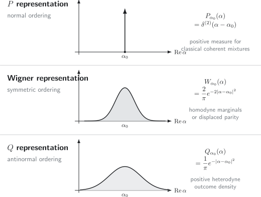
The same coherent state $\lvert\alpha_0\rangle$ in three representations. The Glauber–Sudarshan distribution is a delta measure, the Wigner function is a vacuum-width Gaussian, and the Husimi function is a broader positive Gaussian. The representations carry different ordering and measurement rules even though they encode the same density operator.

Glauber–Sudarshan P representation

The diagonal coherent-state representation is

$$\rho = \int_{\mathbb C}d^2\alpha\, P(\alpha) \lvert\alpha\rangle \langle\alpha\rvert.$$

If $P$ is a nonnegative normalized measure, the state is a statistical mixture of coherent states. This is the standard optical classicality criterion because each coherent component behaves like a classical complex amplitude for normally ordered photodetection correlations.

The word “measure” matters. For a coherent state,

$$P_{\alpha_0}(\alpha) = \delta^{(2)} \left( \alpha-\alpha_0 \right),$$

which is singular as a function but perfectly acceptable as a positive probability measure. A claim that every singular $P$ is nonclassical is therefore false. Number states and squeezed states require more singular generalized distributions that cannot be interpreted as nonnegative measures.

The $P$ representation is adapted to normal ordering:

$$\left\langle (\hat a^\dagger)^m \hat a^n \right\rangle = \int d^2\alpha\, P(\alpha) (\alpha^*)^m \alpha^n.$$

This identity connects positive-$P$ classicality directly to counting statistics and intensity correlations. It does not mean that a singular $P$ can be sampled pointwise in an experiment.

Wigner representation

The Wigner distribution is the symmetrically ordered member of the family. In the optical amplitude convention used here, its displaced-parity form is

$$W(\alpha) = \frac{2}{\pi} \operatorname{Tr} \left[ \hat D^\dagger(\alpha) \rho \hat D(\alpha) \hat\Pi \right],$$

where

$$\hat\Pi = (-1)^{\hat a^\dagger\hat a}$$

is photon-number parity. The formula immediately gives the bound

$$-\frac{2}{\pi} \leq W(\alpha) \leq \frac{2}{\pi}$$

for a single mode, because parity has eigenvalues $\pm1$.

For a coherent state,

$$W_{\alpha_0}(\alpha) = \frac{2}{\pi} \exp\left[ -2\lvert\alpha-\alpha_0\rvert^2 \right].$$

Its center gives the mean complex amplitude, while its width is the vacuum uncertainty required by the commutator. The function is not an ordinary joint probability for sharp $X$ and $P$, even when it happens to be nonnegative.

Symmetric products are phase-space moments. For example,

$$\left\langle \frac{ \hat a^\dagger\hat a + \hat a\hat a^\dagger }{2} \right\rangle = \int d^2\alpha\, W(\alpha) \lvert\alpha\rvert^2.$$

Since

$$\frac{ \hat a^\dagger\hat a + \hat a\hat a^\dagger }{2} = \hat n+\frac12,$$

the mean photon number is

$$\langle\hat n\rangle = \int d^2\alpha\, W(\alpha) \left( \lvert\alpha\rvert^2 - \frac12 \right).$$

The subtraction is the vacuum half quantum. Omitting it is one of the most common ordering mistakes.

Husimi Q representation

Coherent states resolve the identity:

$$\int_{\mathbb C} \frac{d^2\alpha}{\pi} \lvert\alpha\rangle \langle\alpha\rvert = I.$$

The Husimi function is

$$Q(\alpha) = \frac{1}{\pi} \langle\alpha\rvert \rho \lvert\alpha\rangle.$$

It obeys

$$Q(\alpha)\geq0, \qquad \int d^2\alpha\,Q(\alpha)=1.$$

These properties have a direct measurement interpretation: $Q$ is the outcome density of the coherent-state positive-operator-valued measure. An ideal heterodyne measurement realizes this POVM. The returned complex amplitude includes an irreducible vacuum-scale uncertainty, so $Q$ is not a joint distribution for two sharp noncommuting quadratures.

For a coherent state,

$$Q_{\alpha_0}(\alpha) = \frac{1}{\pi} \exp\left[ -\lvert\alpha-\alpha_0\rvert^2 \right].$$

Antinormally ordered moments follow from $Q$:

$$\left\langle \hat a^n (\hat a^\dagger)^m \right\rangle = \int d^2\alpha\, Q(\alpha) \alpha^n (\alpha^*)^m.$$

In particular,

$$\int d^2\alpha\, Q(\alpha) \lvert\alpha\rvert^2 = \langle\hat a\hat a^\dagger\rangle = \langle\hat n\rangle+1,$$

so

$$\langle\hat n\rangle = \int d^2\alpha\, Q(\alpha) \left( \lvert\alpha\rvert^2-1 \right).$$

The larger subtraction reflects the added heterodyne vacuum noise.

One State, Three Symbols

The same operator can require different c-number symbols depending on the distribution used for the state. For the number operator,

State representation	Matching symbol for $\hat n$	Average
$P(\alpha)$	$\lvert\alpha\rvert^2$	normal ordering
$W(\alpha)$	$\lvert\alpha\rvert^2-1/2$	symmetric ordering
$Q(\alpha)$	$\lvert\alpha\rvert^2-1$	antinormal ordering

Every row gives the same $\langle\hat n\rangle$ when the matching pair is used. Combining $Q$ with the normal symbol $\lvert\alpha\rvert^2$ would overestimate the occupation by one photon; combining $W$ with it would overestimate by one half.

The general rule is not “integrate the classical expression against whichever distribution is convenient.” It is “transform the state and observable using dual ordering conventions.”

Gaussian Smoothing Hierarchy

For $s'<s$, the less ordered distribution is a Gaussian convolution of the more ordered one:

$$\begin{aligned} W^{(s')}(\alpha) &= \frac{2}{\pi(s-s')} \int d^2\beta\, W^{(s)}(\beta) \\ &\quad\times \exp\left[ -\frac{ 2\lvert\alpha-\beta\rvert^2 }{ s-s' } \right]. \end{aligned}$$

Thus

$$P \longrightarrow W \longrightarrow Q$$

adds vacuum-scale Gaussian blur at each step. Directly,

$$Q(\alpha) = \frac{1}{\pi} \int d^2\beta\, P(\beta) e^{-\lvert\alpha-\beta\rvert^2}.$$

The smoothing hierarchy explains several facts at once:

• a singular $P$ can yield a regular Wigner function;
• Wigner interference fringes can disappear in $Q$;
• $Q$ is nonnegative for every state;
• reconstructing $P$ from noisy $Q$ data requires Gaussian deconvolution and is usually severely ill-conditioned.

Smoothing is not loss of information in the exact mathematical representation: each characteristic function determines the density operator. It is a practical loss of robustness because inversion amplifies high-frequency statistical and calibration noise.

State Atlas

The representation hierarchy becomes concrete by comparing standard optical states.

Vacuum and coherent states

Vacuum is the coherent state with $\alpha_0=0$:

$$P_0(\alpha)=\delta^{(2)}(\alpha),$$ $$W_0(\alpha) = \frac{2}{\pi} e^{-2\lvert\alpha\rvert^2},$$

and

$$Q_0(\alpha) = \frac{1}{\pi} e^{-\lvert\alpha\rvert^2}.$$

Displacement translates each representation without changing its shape:

$$F_{\hat D(\alpha_0) \rho \hat D^\dagger(\alpha_0)}(\alpha) = F_\rho(\alpha-\alpha_0),$$

for $F=P,W,Q$. This covariance is why the complex plane is so useful for laser-like fields and linear optical networks.

Thermal light

A one-mode thermal state with mean occupation $\bar n>0$ has the positive Glauber–Sudarshan density

$$P_{\mathrm{th}}(\alpha) = \frac{1}{\pi\bar n} \exp\left( -\frac{\lvert\alpha\rvert^2}{\bar n} \right).$$

Its Wigner and Husimi functions are

$$W_{\mathrm{th}}(\alpha) = \frac{2}{ \pi(2\bar n+1) } \exp\left[ -\frac{ 2\lvert\alpha\rvert^2 }{ 2\bar n+1 } \right],$$

and

$$Q_{\mathrm{th}}(\alpha) = \frac{1}{ \pi(\bar n+1) } \exp\left[ -\frac{ \lvert\alpha\rvert^2 }{ \bar n+1 } \right].$$

All are rotationally symmetric because the state has no phase preference. All are nonnegative, and the positive $P$ shows that ideal thermal light is classical under the coherent-mixture criterion despite its super-Poissonian counting and bunching.

Number states

For the number state $\lvert n\rangle$,

$$W_n(\alpha) = \frac{2}{\pi} (-1)^n L_n\left( 4\lvert\alpha\rvert^2 \right) e^{-2\lvert\alpha\rvert^2},$$

where $L_n$ is a Laguerre polynomial. At the origin,

$$W_n(0) = \frac{2}{\pi}(-1)^n,$$

which is the parity rule. Every odd number state is maximally negative at the origin in this normalization.

The corresponding Husimi function is

$$Q_n(\alpha) = \frac{ e^{-\lvert\alpha\rvert^2} \lvert\alpha\rvert^{2n} }{ \pi n! }.$$

It is nonnegative and has a zero of order $2n$ at the origin for $n>0$. The $P$ representation is a finite combination of derivatives of a delta distribution and is not a nonnegative measure.

Squeezed Gaussian states

A squeezed vacuum has an elliptical, nonnegative Gaussian Wigner function. In the quadrature convention used here, its covariance eigenvalues are

$$V_- = \frac12e^{-2r}, \qquad V_+ = \frac12e^{2r}.$$

The Husimi function is a broader positive ellipse because it includes the coherent-state measurement noise. The Glauber–Sudarshan representation is not a nonnegative measure whenever one quadrature variance falls below the vacuum value. This example is the standard warning that Wigner positivity does not imply optical classicality.

The covariance formulas and multimode Gaussian machinery are canonical on Gaussian States and Wigner Functions. The generation, calibration, and loss budget are developed on Squeezed Light.

Coherent superpositions

For an even or odd superposition

$$\lvert\psi_\pm\rangle \propto \lvert\alpha_0\rangle \pm \lvert-\alpha_0\rangle,$$

the Wigner function contains two positive lobes and an oscillatory interference term between them. Negative fringes encode the relative phase; the incoherent mixture of the two coherent states lacks those fringes.

The $Q$ function smooths the fringes and remains nonnegative. It can still distinguish the coherent superposition from the mixture when measured with enough precision, because positivity does not mean absence of phase information. The $P$ representation is highly singular and nonclassical.

Compact comparison

Coherent state. $P$ is a positive delta measure, $W$ is a positive vacuum-width Gaussian, and $Q$ is a broader positive Gaussian.

Thermal state. All three are positive Gaussians, with widths increased in the order $P$, $W$, $Q$.

Squeezed vacuum. $P$ is a nonclassical generalized distribution, $W$ is a positive ellipse, and $Q$ is a broader positive ellipse.

Number state. $P$ is derivative-like and singular, $W$ oscillates and is negative for $n>0$, and $Q$ is a positive ring-like density.

Coherent superposition. $P$ is singular and nonclassical, $W$ contains interference fringes and can be negative, and $Q$ is smooth and positive.

No single column by itself is “more quantum.” Each emphasizes a different ordering and experimental question.

How the Distributions Are Measured

A phase-space representation is not automatically a histogram of detector outcomes. The measurement map must be stated. Three standard routes have especially clean meanings.

Homodyne marginals and Wigner tomography

Balanced homodyne detection measures one rotated quadrature

$$\hat X_\theta = \hat X\cos\theta + \hat P\sin\theta$$

selected by the local-oscillator phase. To write its marginal without hidden Jacobians, define the Wigner density normalized in the real quadratures by

$$W_{XP}(X,P) = \frac12 W\left( \frac{X+iP}{\sqrt2} \right).$$

Then

$$\int dX\,dP\,W_{XP}(X,P)=1.$$

With the rotated conjugate coordinate

$$P_\theta = -X\sin\theta + P\cos\theta,$$

the measured probability density is the line marginal

$$p_\theta(x) = \int_{-\infty}^{\infty} dP_\theta\, W_{XP}(x,P_\theta).$$

Every $p_\theta$ is nonnegative even when $W$ has negative regions. By collecting quadrature samples over $0\leq\theta<\pi$, one obtains the Radon projections needed to reconstruct the Wigner function or density matrix.

An inverse Radon transform is exact only for ideal continuous data. Real optical tomography must address:

• finite sample size and phase coverage;
• detector efficiency and electronic noise;
• local-oscillator mode matching;
• finite digitizer range and binning;
• filtering, regularization, or a finite reconstruction basis;
• positivity and normalization constraints on the inferred density operator.

Filtered back-projection can display the geometry directly, while maximum-likelihood or Bayesian state estimation can enforce a physical density operator. Different estimators can produce visibly different small features at finite data size. A negative patch is compelling only when it is stable against the stated uncertainty and reconstruction choices.

Homodyne and Heterodyne Detection owns the practical receiver, mode selection, vacuum calibration, and optical quadrature POVM. The open-systems Homodyne Detection page owns continuous stochastic records. The present page uses calibrated quadrature distributions as phase-space projections.

Heterodyne detection and Q sampling

The coherent-state POVM has elements

$$E(\alpha)\,d^2\alpha = \frac{d^2\alpha}{\pi} \lvert\alpha\rangle \langle\alpha\rvert.$$

Its outcome probability is

$$p(\alpha) = \operatorname{Tr} \left[ \rho E(\alpha) \right] =Q(\alpha).$$

Ideal heterodyne detection therefore samples $Q$ directly. Optical heterodyne receivers use a frequency-offset local oscillator; dual-homodyne receivers split the signal and measure orthogonal quadratures. In both pictures an unused port or image band introduces the vacuum noise required by simultaneous two-quadrature readout.

The raw histogram equals the ideal $Q$ function only after the complex gain, offset, phase convention, image-band response, and efficiency have been calibrated. Added amplifier noise in microwave receivers broadens the histogram beyond the ideal coherent-state POVM. Calling every IQ histogram a Husimi function without specifying that noise model is too strong.

Homodyne and Heterodyne Detection owns the frequency-offset receiver, image-band vacuum, calibration, and coherent-state POVM. The open-systems Heterodyne Detection owns the two-Wiener record and conditional-state description.

Displacement followed by parity

The displaced-parity identity provides a pointwise route to the Wigner function. Displace the state by $-\alpha$, resolve the photon-number probabilities $p_n(\alpha)$, and form

$$W(\alpha) = \frac{2}{\pi} \sum_{n=0}^{\infty} (-1)^n p_n(\alpha).$$

The procedure does not require an inverse Radon transform. It does require a calibrated displacement, photon-number resolution over enough of the distribution, and tight control of loss because parity is highly sensitive to missed photons.

Variants are used in cavity and circuit QED, trapped-ion motional-state measurements, and optical photon-counting experiments. The physical apparatus differs, but the mathematical observable is displaced parity.

Why P is rarely plotted from raw samples

The Glauber–Sudarshan representation is most naturally accessed through normally ordered moments and inequalities rather than pointwise sampling. Photocount correlations estimate quantities such as

$$\left\langle (\hat a^\dagger)^m \hat a^m \right\rangle,$$

which are ordinary moments of a positive $P$ if such a measure exists. Violations of inequalities obeyed by every classical random intensity then witness a nonclassical $P$.

In principle, complete tomographic data determine $P$. In practice, obtaining it from $W$ or $Q$ reverses Gaussian smoothing and can turn small high-frequency noise into enormous oscillations. A regularized surrogate must not be described as the unique raw $P$ distribution without its bandwidth or prior.

Operational dictionary

Glauber–Sudarshan $P$. Its natural ordering is normal. Photodetection moments and positive-$P$ classicality tests are the main experimental connections; the distribution itself may be generalized rather than pointwise plottable.

Wigner $W$. Its natural ordering is symmetric. Homodyne marginals and displaced parity provide experimental access; the function can be negative, and full homodyne tomography is an inverse problem.

Husimi $Q$. Its natural ordering is antinormal. Ideal heterodyne outcomes sample it directly; it is always positive and includes vacuum broadening.

Loss, Efficiency, and Added Noise

Loss does more than lower a plotted amplitude. It mixes the selected mode with an environmental mode and changes the state.

Pure-loss channel

A pure-loss channel of transmissivity $\eta$ is modeled by

$$\hat a_{\mathrm{out}} = \sqrt\eta\, \hat a_{\mathrm{in}} + \sqrt{1-\eta}\, \hat v,$$

where $\hat v$ is an environmental vacuum mode. It transforms the first moment as

$$\langle\hat a\rangle_{\mathrm{out}} = \sqrt\eta\, \langle\hat a\rangle_{\mathrm{in}},$$

and a one-mode quadrature covariance matrix as

$$V_{\mathrm{out}} = \eta V_{\mathrm{in}} + (1-\eta) \frac{I_2}{2}.$$

For the ordered characteristic functions,

$$\begin{aligned} \chi_{s,\mathrm{out}}(\xi) &= \chi_{s,\mathrm{in}} \left( \sqrt\eta\,\xi \right) \\ &\quad\times \exp\left[ -\frac{ (1-s)(1-\eta) }{2} \lvert\xi\rvert^2 \right]. \end{aligned}$$

The $P$ characteristic function with $s=1$ receives no extra Gaussian factor; a positive coherent-state mixture remains a positive coherent-state mixture with contracted amplitudes. The Wigner and $Q$ functions acquire vacuum smoothing as well as contraction. Nonclassical structure can therefore become invisible after enough loss.

Example: one photon under loss

An incident one-photon state becomes

$$\rho_{\mathrm{out}} = \eta \lvert1\rangle\langle1\rvert + (1-\eta) \lvert0\rangle\langle0\rvert.$$

At the origin,

$$\begin{aligned} W_{\mathrm{out}}(0) &= \frac{2}{\pi} \left[ (1-\eta)-\eta \right] \\ &= \frac{2}{\pi} (1-2\eta). \end{aligned}$$

The measured state retains Wigner negativity at the origin only when

$$\eta>\frac12.$$

For lower efficiency the Wigner function can be everywhere nonnegative even though the input was a number state. Absence of observed negativity is not proof that the source emitted a classical state.

Detector correction versus measured state

There are two legitimate but different reporting choices:

1. reconstruct the state arriving at the detector, including propagation and detection loss;
2. infer an upstream source state by inverting a calibrated channel model.

The second can be scientifically useful, but it is model dependent and often ill-conditioned. A mature report labels raw and corrected quantities, propagates efficiency uncertainty, states the regularization, and verifies the inferred density operator against independent observables.

An efficiency correction that merely sharpens a plot until negativity appears is not evidence by itself.

Mode mismatch is loss plus possible contamination

Homodyne and heterodyne receivers project the signal onto the local-oscillator mode. If the normalized signal mode is $f$ and the analyzed mode is $g$, the overlap

$$\mu = \langle g,f\rangle$$

sets an effective efficiency $\lvert\mu\rvert^2$ only when unmatched modes are equivalent to vacuum and are not otherwise detected. Background light, orthogonal populated modes, phase drift, or correlated technical noise can add contamination rather than pure vacuum loss.

The quoted phase-space distribution always belongs to the analyzed mode $g$. This is why mode declarations are part of the state definition, not merely an experimental footnote.

Multimode and Pulsed Fields

For $M$ declared modes, collect the amplitudes into

$$\boldsymbol\alpha = (\alpha_1,\ldots,\alpha_M)^{\mathsf T}.$$

A multimode distribution is normalized over

$$d^{2M}\boldsymbol\alpha = \prod_{j=1}^{M}d^2\alpha_j.$$

The coherent-state representation becomes

$$\rho = \int d^{2M}\boldsymbol\alpha\, P(\boldsymbol\alpha) \lvert\boldsymbol\alpha\rangle \langle\boldsymbol\alpha\rvert.$$

Passive linear optics applies a unitary mode transformation

$$\boldsymbol{\hat a}_{\mathrm{out}} = U \boldsymbol{\hat a}_{\mathrm{in}},$$

and rotates coherent amplitudes according to

$$\boldsymbol\alpha_{\mathrm{out}} = U \boldsymbol\alpha_{\mathrm{in}}.$$

The full phase-space distribution is transformed by the corresponding linear change of coordinates. A reduced one-mode distribution is obtained by integrating over all unobserved mode amplitudes. This marginalization can hide correlations, entanglement, and joint negativity.

Pulsed homodyne modes

A pulsed local oscillator defines a temporal supermode

$$\hat a_g = \int dt\, g^*(t) \hat a(t), \qquad \int dt\,\lvert g(t)\rvert^2=1.$$

The measured quadrature samples and reconstructed Wigner function refer to that operator. Changing the pulse shape $g(t)$ changes the mode and therefore the reduced state. Principal-component or mode-function analyses can identify the supermodes carrying the nonclassical structure, but the resulting basis must be reported.

Continuous-wave sidebands

A continuous-wave homodyne record analyzed near a radio-frequency offset can involve upper and lower optical sidebands jointly. Depending on the demodulation phase and filter, the effective observables may be quadratures of a symmetric or antisymmetric sideband supermode rather than of one isolated frequency mode.

An ellipse plotted from a noise spectrum is not automatically the Wigner function of a single carrier mode. The temporal filter, sideband pairing, and normalization determine which canonical mode is represented.

Classicality and Negativity

The implications among the three common positivity conditions are one-way:

$$\begin{gathered} \text{positive }P \Longrightarrow W\geq0, \\ W\geq0 \Longrightarrow Q\geq0. \end{gathered}$$

The final condition holds for every quantum state, so it is not a classicality test. Neither converse is valid.

Positive P is the optical classical set

If $P$ is a nonnegative measure, then

$$\rho = \int d^2\alpha\, P(\alpha) \lvert\alpha\rangle \langle\alpha\rvert$$

is a convex mixture of coherent states. Normally ordered moments then equal moments of an ordinary classical random complex amplitude. Classical inequalities for intensity fluctuations follow.

For example, every positive-$P$ one-mode state satisfies

$$\operatorname{Var}(X_\theta) \geq \frac12,$$

because each coherent component contributes vacuum variance $1/2$ and classical mixing can only add variance of the component means. Quadrature squeezing below vacuum therefore certifies failure of a positive Glauber–Sudarshan measure.

Likewise, under the stated single-mode and detector assumptions,

$$g^{(2)}(0)<1$$

or a sub-Poissonian Fano factor certifies nonclassicality. These witnesses can detect states whose Wigner functions remain nonnegative.

Wigner negativity is sufficient, not necessary

If $W$ is negative anywhere, the state cannot have a positive $P$, because Gaussian smoothing of a positive measure cannot create negative values. Wigner negativity is therefore a sufficient witness of optical nonclassicality.

It is not necessary. Squeezed Gaussian states and many entangled Gaussian states have nonnegative Wigner functions. For pure continuous-variable states, Hudson’s theorem makes the boundary sharp: under its regularity assumptions, a pure state has a nonnegative Wigner function only if it is Gaussian. Mixed non-Gaussian states can nevertheless have positive Wigner functions.

A common negativity volume is

$$\mathcal N_W = \frac12 \left[ \int d^2\alpha\, \lvert W(\alpha)\rvert -1 \right].$$

Its numerical value depends on the normalized state but not on a harmless linear rescaling of coordinates when the integration measure is transformed consistently. Its uncertainty can be strongly estimator dependent in finite tomography.

Q positivity is not classicality

Every density operator gives

$$Q(\alpha) = \frac{1}{\pi} \langle\alpha\rvert\rho\lvert\alpha\rangle \geq0.$$

The positivity reflects positivity of a POVM outcome probability. Number states, coherent superpositions, and squeezed states all have positive $Q$ functions. Nonclassical information remains encoded in their shapes, zeros, moments, and incompatibility with any positive-$P$ model, but not in negative $Q$ values.

Nonclassicality is not the same as entanglement

A single-mode squeezed state is nonclassical without being entangled across the declared one-mode tensor factor. Sending it and vacuum through a beam splitter can produce two-mode entanglement. Conversely, whether a multimode state is separable depends on the subsystem split, while positive-$P$ classicality asks whether it is a mixture of multimode coherent products in a specified mode basis.

The concepts are related through optical transformations but should not be used interchangeably.

A Reliable Analysis Workflow

For an optical phase-space claim, proceed in this order.

1. Define the mode and reference phase

Specify the spatial, temporal, spectral, and polarization mode. State how its phase is fixed relative to a local oscillator or pump.

2. Fix normalization

Write the quadrature operators, vacuum variance, relation to $\alpha$, and the measure used to normalize the distribution.

3. Name the measured observable

Distinguish homodyne quadrature samples, heterodyne complex outcomes, photon-number-resolved displaced parity, and normally ordered count correlations.

4. State the forward detector model

Include propagation loss, quantum efficiency, electronic or amplifier noise, mode overlap, phase noise, finite bandwidth, and any binning or filtering.

5. Reconstruct only what the data support

State the estimator, truncation, regularization, prior, or kernel bandwidth. Check positivity and trace of the density matrix when one is reconstructed.

6. Validate against independent summaries

Compare reconstructed moments with directly estimated means, variances, photon counts, or correlations. Verify that integrating the Wigner function reproduces observed homodyne marginals.

7. Phrase the conclusion at the right level

Examples include:

• “the detector-plane Wigner function is negative with stated uncertainty”;
• “the loss-corrected source model is inconsistent with every positive-$P$ state”;
• “the measured quadrature variance is below the calibrated vacuum level”;
• “the heterodyne histogram agrees with the predicted noisy $Q$ model.”

These are stronger and more reproducible than saying only that a plot “looks quantum.”

Common Mistakes

• Treating $\alpha$ as a physical electric field without the selected mode’s normalization factor.
• Comparing widths from sources that use different quadrature conventions.
• Forgetting that $d^2\alpha=dX\,dP/2$ in the convention used here.
• Calling a Wigner function an ordinary joint probability for sharp quadratures.
• Calling every singular $P$ nonclassical; a coherent state’s delta measure is positive.
• Assuming positive Wigner implies positive Glauber–Sudarshan $P$.
• Treating positive $Q$ as evidence of classicality.
• Extracting moments with an ordering symbol that does not match the state distribution.
• Calling an uncalibrated IQ histogram the ideal Husimi function.
• Interpreting a noise ellipse for unspecified sidebands as a complete one-mode Wigner function.
• Correcting loss without reporting the forward model, uncertainty, and regularization.
• Reading small reconstructed ripples as negativity without a statistical stability test.
• Tracing out unmeasured modes and then making claims about the full multimode state.

Connections

• Quantum Optics supplies the state–transformation–measurement map for the chapter.
• Photon Number States develops the number basis, parity, and direct-counting interpretation.
• Coherent Light develops the optical meaning of $\alpha$ and the positive-$P$ reference state.
• Thermal Light develops the positive Gaussian mixture and bunching of chaotic fields.
• Squeezed Light develops positive-Wigner but nonclassical Gaussian optical states.
• Beam Splitters develops the passive mode unitary behind loss dilations, homodyne mixing, and optical phase-space rotations.
• Wigner Function owns the general density-operator transform and standard canonical examples.
• Marginals and Quasi-Probabilities owns the general relation among marginals, negativity, $P$, $W$, and $Q$.
• Coherent States in Phase Space owns displacement geometry and coherent-state Wigner evolution.
• Gaussian States and Wigner Functions owns covariance matrices, symplectic transformations, and multimode Gaussian formulas.
• Phase-Space Conventions is the reference sheet for Weyl symbols, trace measures, and signs.
• Homodyne Detection and Heterodyne Detection develop the corresponding detector records and stochastic descriptions.

Exercises

1. Coordinate measure and vacuum marginal

Using

$$\alpha=\frac{X+iP}{\sqrt2},$$

show that $d^2\alpha=dX\,dP/2$. Convert

$$W_0(\alpha) = \frac{2}{\pi} e^{-2\lvert\alpha\rvert^2}$$

to the normalized real-quadrature density and recover the vacuum probability density for $X$.

Solution

The real and imaginary parts are

$$\operatorname{Re}\alpha = \frac{X}{\sqrt2}, \qquad \operatorname{Im}\alpha = \frac{P}{\sqrt2}.$$

The Jacobian is therefore $1/2$:

$$d^2\alpha = d(\operatorname{Re}\alpha) d(\operatorname{Im}\alpha) = \frac12\,dX\,dP.$$

Since

$$\lvert\alpha\rvert^2 = \frac{X^2+P^2}{2},$$

the density normalized with respect to $dX\,dP$ is

$$\begin{aligned} W_{XP,0}(X,P) &= \frac12W_0(\alpha) \\ &= \frac{1}{\pi} e^{-(X^2+P^2)}. \end{aligned}$$

Integrating over $P$ gives

$$\begin{aligned} p_0(X) &= \int_{-\infty}^{\infty} dP\,W_{XP,0}(X,P) \\ &= \frac{e^{-X^2}}{\pi} \int_{-\infty}^{\infty} dP\,e^{-P^2} \\ &= \frac{1}{\sqrt\pi} e^{-X^2}. \end{aligned}$$

This Gaussian has variance $1/2$, as required by the chosen quadrature normalization.

2. Smoothing a coherent-state P distribution

Starting from

$$P_{\alpha_0}(\beta) = \delta^{(2)}(\beta-\alpha_0),$$

use the Gaussian smoothing relation to derive the coherent-state Wigner and Husimi functions.

Solution

For $s=1$ and $s'=0$,

$$W(\alpha) = \frac{2}{\pi} \int d^2\beta\, P(\beta) e^{-2\lvert\alpha-\beta\rvert^2}.$$

The delta measure sets $\beta=\alpha_0$:

$$W_{\alpha_0}(\alpha) = \frac{2}{\pi} e^{-2\lvert\alpha-\alpha_0\rvert^2}.$$

For $s=1$ and $s'=-1$,

$$Q(\alpha) = \frac{1}{\pi} \int d^2\beta\, P(\beta) e^{-\lvert\alpha-\beta\rvert^2},$$

so

$$Q_{\alpha_0}(\alpha) = \frac{1}{\pi} e^{-\lvert\alpha-\alpha_0\rvert^2}.$$

The $Q$ distribution is broader because it contains one additional Gaussian smoothing step.

3. Mean occupation in all three representations

For a coherent state $\lvert\alpha_0\rangle$, evaluate the phase-space formulas for $\langle\hat n\rangle$ using $P$, $W$, and $Q$. Explain why the three different symbols give one answer.

Solution

The positive delta measure gives immediately

$$\int d^2\alpha\, P(\alpha) \lvert\alpha\rvert^2 = \lvert\alpha_0\rvert^2.$$

The coherent-state Wigner Gaussian has

$$\int d^2\alpha\, W(\alpha) \lvert\alpha\rvert^2 = \lvert\alpha_0\rvert^2 + \frac12.$$

Therefore its symmetric symbol gives

$$\int d^2\alpha\, W(\alpha) \left( \lvert\alpha\rvert^2-\frac12 \right) = \lvert\alpha_0\rvert^2.$$

Similarly, the $Q$ Gaussian has

$$\int d^2\alpha\, Q(\alpha) \lvert\alpha\rvert^2 = \lvert\alpha_0\rvert^2+1,$$

so

$$\int d^2\alpha\, Q(\alpha) \left( \lvert\alpha\rvert^2-1 \right) = \lvert\alpha_0\rvert^2.$$

The offsets are the vacuum corrections associated with normal, symmetric, and antinormal ordering. Each distribution must be paired with its matching operator symbol.

4. Thermal broadening

Verify from the three thermal distributions that

$$\langle\lvert\alpha\rvert^2\rangle_P = \bar n, \qquad \langle\lvert\alpha\rvert^2\rangle_W = \bar n+\frac12,$$

and

$$\langle\lvert\alpha\rvert^2\rangle_Q = \bar n+1.$$

Solution

A normalized circular Gaussian

$$G_v(\alpha) = \frac{1}{\pi v} e^{-\lvert\alpha\rvert^2/v}$$

satisfies

$$\int d^2\alpha\, G_v(\alpha) \lvert\alpha\rvert^2 =v.$$

The thermal $P$ distribution has $v=\bar n$. Rewriting the Wigner function as

$$W_{\mathrm{th}}(\alpha) = \frac{1}{ \pi(\bar n+1/2) } \exp\left[ -\frac{ \lvert\alpha\rvert^2 }{ \bar n+1/2 } \right]$$

shows $v=\bar n+1/2$. The Husimi function has $v=\bar n+1$.

Subtracting the ordering offsets $0$, $1/2$, and $1$ gives the same physical mean occupation $\bar n$ in every representation.

5. Parity at the origin

Use displaced parity to show that

$$W_n(0) = \frac{2}{\pi}(-1)^n$$

for a number state. Why does this make the origin especially useful for odd states?

Solution

At $\alpha=0$, no displacement is applied. Since

$$\hat\Pi\lvert n\rangle = (-1)^n\lvert n\rangle,$$

the displaced-parity identity gives

$$\begin{aligned} W_n(0) &= \frac{2}{\pi} \langle n\rvert \hat\Pi \lvert n\rangle \\ &= \frac{2}{\pi}(-1)^n. \end{aligned}$$

Every odd number state reaches the minimum allowed one-mode value $-2/\pi$ at the origin. A calibrated parity measurement there is therefore a direct negativity test, although loss can rapidly reduce the contrast.

6. Positive P forbids quadrature squeezing

Prove that every state with a nonnegative Glauber–Sudarshan measure satisfies

$$\operatorname{Var}(X_\theta)\geq\frac12.$$

Solution

For a coherent component $\lvert\alpha\rangle$,

$$\operatorname{Var}_\alpha(X_\theta) = \frac12.$$

Its mean is the real classical quantity

$$x_\theta(\alpha) = \sqrt2 \operatorname{Re} \left( \alpha e^{-i\theta} \right).$$

For a positive mixture $P(\alpha)$, the law of total variance gives

$$\begin{aligned} \operatorname{Var}(X_\theta) &= \int d^2\alpha\, P(\alpha) \operatorname{Var}_\alpha(X_\theta) \\ &\quad+ \operatorname{Var}_P \left[ x_\theta(\alpha) \right] \\ &= \frac12 + \operatorname{Var}_P \left[ x_\theta(\alpha) \right] \geq \frac12. \end{aligned}$$

Therefore any verified variance below vacuum rules out every nonnegative coherent-state mixture, even though the squeezed state’s Wigner function can remain positive.

7. One photon through loss

Derive the output state and origin value of the Wigner function when a one-photon state passes through a pure-loss channel. Find the efficiency threshold for observed negativity.

Solution

The beam-splitter dilation acts as

$$\begin{aligned} \lvert1\rangle_a\lvert0\rangle_v &\longmapsto \sqrt\eta\, \lvert1\rangle_a\lvert0\rangle_v \\ &\quad+ \sqrt{1-\eta}\, \lvert0\rangle_a\lvert1\rangle_v. \end{aligned}$$

Tracing out the environment removes the coherence between orthogonal environment states:

$$\rho_{\mathrm{out}} = \eta\lvert1\rangle\langle1\rvert + (1-\eta) \lvert0\rangle\langle0\rvert.$$

Using the parity values,

$$\begin{aligned} W_{\mathrm{out}}(0) &= \eta\left(-\frac{2}{\pi}\right) + (1-\eta) \left(\frac{2}{\pi}\right) \\ &= \frac{2}{\pi}(1-2\eta). \end{aligned}$$

It is negative exactly when $\eta>1/2$. Below this threshold the input state was still nonclassical, but origin negativity is no longer visible in the detector-plane state.

8. Choosing a reconstruction route

You must characterize an unknown pulsed optical state. Compare the information and leading vulnerabilities of three choices: phase-scanned homodyne tomography, heterodyne sampling, and displacement followed by photon-number parity. Which would directly return $Q$, and which can return a Wigner value without a global inverse transform?

Solution

Phase-scanned homodyne detection returns quadrature marginals. With enough local-oscillator phases, those marginals determine the Wigner function or density matrix. Its main practical vulnerabilities are phase calibration, mode matching, efficiency, and instability or bias in the tomographic inverse.

Ideal heterodyne detection returns complex outcomes distributed according to $Q$. It samples both quadratures in each shot but includes irreducible vacuum noise. Added receiver noise and complex-gain calibration must be included in a realistic model.

Displacement followed by photon-number resolution returns displaced parity, and hence one Wigner value, directly from the even-minus-odd probability. It avoids a global Radon inversion but is especially sensitive to photon loss, number-resolution limits, and displacement calibration.

Thus heterodyne directly returns $Q$, while displaced parity can return $W(\alpha)$ point by point without a global inverse transform. Homodyne is often the most flexible route to a full continuous-variable state when a high-quality mode-matched local oscillator is available.

References

1. E. Wigner, “On the Quantum Correction for Thermodynamic Equilibrium,” Physical Review 40, 749–759 (1932), doi:10.1103/PhysRev.40.749.
2. K. Husimi, “Some Formal Properties of the Density Matrix,” Proceedings of the Physico-Mathematical Society of Japan 22, 264–314 (1940).
3. E. C. G. Sudarshan, “Equivalence of Semiclassical and Quantum Mechanical Descriptions of Statistical Light Beams,” Physical Review Letters 10, 277–279 (1963), doi:10.1103/PhysRevLett.10.277.
4. R. J. Glauber, “Coherent and Incoherent States of the Radiation Field,” Physical Review 131, 2766–2788 (1963), doi:10.1103/PhysRev.131.2766.
5. K. E. Cahill and R. J. Glauber, “Ordered Expansions in Boson Amplitude Operators,” Physical Review 177, 1857–1881 (1969), doi:10.1103/PhysRev.177.1857.
6. K. E. Cahill and R. J. Glauber, “Density Operators and Quasiprobability Distributions,” Physical Review 177, 1882–1902 (1969), doi:10.1103/PhysRev.177.1882.
7. R. L. Hudson, “When Is the Wigner Quasi-Probability Density Non-Negative?” Reports on Mathematical Physics 6, 249–252 (1974), doi:10.1016/0034-4877(74)90007-X.
8. M. Hillery, R. F. O’Connell, M. O. Scully, and E. P. Wigner, “Distribution Functions in Physics: Fundamentals,” Physics Reports 106, 121–167 (1984), doi:10.1016/0370-1573(84)90160-1.
9. K. Vogel and H. Risken, “Determination of Quasiprobability Distributions in Terms of Probability Distributions for the Rotated Quadrature Phase,” Physical Review A 40, 2847–2849 (1989), doi:10.1103/PhysRevA.40.2847.
10. D. T. Smithey, M. Beck, M. G. Raymer, and A. Faridani, “Measurement of the Wigner Distribution and the Density Matrix of a Light Mode Using Optical Homodyne Tomography,” Physical Review Letters 70, 1244–1247 (1993), doi:10.1103/PhysRevLett.70.1244.
11. K. Banaszek and K. Wódkiewicz, “Direct Probing of Quantum Phase Space by Photon Counting,” Physical Review Letters 76, 4344–4347 (1996), doi:10.1103/PhysRevLett.76.4344.
12. U. Leonhardt, Measuring the Quantum State of Light, Cambridge University Press (1997).
13. W. P. Schleich, Quantum Optics in Phase Space, Wiley-VCH (2001), doi:10.1002/3527602976.
14. A. I. Lvovsky and M. G. Raymer, “Continuous-Variable Optical Quantum-State Tomography,” Reviews of Modern Physics 81, 299–332 (2009), doi:10.1103/RevModPhys.81.299.
15. D. F. Walls and G. J. Milburn, Quantum Optics, 2nd ed., Springer (2008), doi:10.1007/978-3-540-28574-8.