Beam Splitters

A beam splitter is the elementary two-port mixer of quantum optics. At a fixed optical frequency and for declared spatial, temporal, and polarization modes, an ideal lossless beam splitter applies a unitary transformation to two annihilation operators. The same transformation redistributes classical field amplitudes, one-photon probability amplitudes, multiphoton creation operators, and Gaussian-state moments.

That common algebra does not make all interference effects identical. Single-photon interference combines alternatives for one excitation. Hong–Ou–Mandel interference combines two-photon alternatives and disappears when information in any unresolved degree of freedom makes the photons distinguishable. A beam splitter can also reveal nonclassical input statistics, but it does not by itself create photons or provide a universal test of quantumness.

Three bookkeeping choices must be stated before using a beam-splitter formula:

• which normalized input and output modes define the ports;
• whether the equation transforms operators or states;
• which phases have been assigned to reflection, transmission, and external propagation.

Different phase conventions are physically equivalent when used consistently. Mixing them is not.

Canonical Scope

This page is the canonical home for an ideal optical beam splitter as a two-mode unitary:

• commutator preservation and photon-number conservation;
• the scattering matrix and its unitary generator;
• phase-convention changes by input and output rephasing;
• vacuum, coherent-state, and Fock-state transformations;
• single-photon path amplitudes;
• ideal and partially distinguishable Hong–Ou–Mandel interference;
• the distinction between a lossless two-port model and a lossy device with environmental ports.

Coherent Light owns the detailed coherent-input calculation and the pure-loss channel example. Photon Number States owns source statistics, antibunching, and the distinction between one-photon purity and indistinguishability. Entanglement in Quantum Optics owns the subsystem interpretation of path-mode entanglement. The subsequent Interferometers page owns Mach–Zehnder phase estimation and shot-noise limits.

Ports Are Modes

Input and output operators

Let $\hat a$ and $\hat b$ annihilate photons in two orthogonal input modes, and let $\hat c$ and $\hat d$ describe two orthogonal output modes. Each mode must include all degrees of freedom needed to specify the field:

$$\begin{aligned} \text{mode} ={}& \text{spatial profile} \\ &+ \text{temporal or spectral envelope} \\ &+ \text{polarization}. \end{aligned}$$

For discrete normalized modes,

$$\begin{aligned} [\hat a,\hat a^\dagger] &= [\hat b,\hat b^\dagger] = 1, \\ [\hat a,\hat b] &= [\hat a,\hat b^\dagger] = 0, \end{aligned}$$

and the same relations must hold for $\hat c$ and $\hat d$. An optical bench label alone is not a complete mode definition. A detector may collect many spectral or spatial modes behind one geometric output port.

Write the linear input–output relation as

$$\begin{pmatrix} \hat c\\ \hat d \end{pmatrix} = S \begin{pmatrix} \hat a\\ \hat b \end{pmatrix}.$$

For a passive device, annihilation operators mix only with annihilation operators. A transformation that mixes $\hat a$ with $\hat a^\dagger$ is an active Bogoliubov transformation and requires an energy source such as a pump.

The validity envelope

The two-mode description assumes that the device does not appreciably couple the selected ports to unmodeled radiation, absorption, polarization, or frequency channels. It is often an excellent approximation within a declared bandwidth. Outside that envelope, the coefficients can depend on frequency and polarization:

$$S \longrightarrow S(\omega,\lambda),$$

where $\lambda$ labels polarization or another internal mode. A single pair of numbers $t$ and $r$ should not be used across a broadband pulse unless their variation is negligible over the occupied spectrum.

Bulk dielectric plates, cube beam splitters, fiber couplers, and integrated directional couplers can all realize two-mode mixing. Their electromagnetic boundary conditions differ, but their ideal quantum description reduces to the same unitary mode transformation after the relevant ports and phases have been fixed.

Lossless Two-Mode Scattering

Unitarity from the commutators

If

$$\hat{\boldsymbol a}_{\mathrm{out}} = S \hat{\boldsymbol a}_{\mathrm{in}},$$

then

$$\begin{aligned} [ \hat a_{\mathrm{out},j}, \hat a_{\mathrm{out},k}^\dagger ] &= \sum_{\mu,\nu} S_{j\mu} S_{k\nu}^* [ \hat a_{\mathrm{in},\mu}, \hat a_{\mathrm{in},\nu}^\dagger ] \\ &= (SS^\dagger)_{jk}. \end{aligned}$$

Canonical output commutators therefore require

$$SS^\dagger=I.$$

For equal numbers of finite input and output modes, $S$ is unitary. This is the quantum version of power conservation for a lossless passive network.

A convenient SU(2) convention

Throughout this page, use

$$\begin{pmatrix} \hat c\\ \hat d \end{pmatrix} = \begin{pmatrix} t&r\\ -r^*&t^* \end{pmatrix} \begin{pmatrix} \hat a\\ \hat b \end{pmatrix},$$

with

$$|t|^2+|r|^2=1.$$

Define the intensity transmittance and reflectance by

$$T=|t|^2, \qquad R=|r|^2, \qquad T+R=1.$$

This matrix has unit determinant. A general $U(2)$ matrix differs only by an overall phase, which can be assigned to the output modes and does not change isolated counting probabilities.

A useful parameterization is

$$\begin{gathered} t=\cos\theta, \qquad r=e^{i\phi}\sin\theta, \\ 0\leq\theta\leq\frac{\pi}{2}. \end{gathered}$$

The balanced case has

$$\theta=\frac{\pi}{4}, \qquad T=R=\frac12.$$

The inverse operator relation is

$$\begin{pmatrix} \hat a\\ \hat b \end{pmatrix} = \begin{pmatrix} t^*&-r\\ r^*&t \end{pmatrix} \begin{pmatrix} \hat c\\ \hat d \end{pmatrix}.$$

That inverse matters when an input state is rewritten in the output Fock basis.

Number conservation

The total photon number is

$$\hat N = \hat a^\dagger\hat a + \hat b^\dagger\hat b.$$

Using $S^\dagger S=I$ gives

$$\hat c^\dagger\hat c + \hat d^\dagger\hat d = \hat N.$$

An ideal passive beam splitter changes how occupation is distributed between ports but preserves total occupation exactly. Energy is conserved as well when the mixed modes have the same carrier frequency. Frequency-converting devices require a more explicit energy ledger even if an effective mode transformation looks unitary.

The Quantum Unitary

Generator

The mode transformation can be generated by

$$\hat U_{\mathrm{BS}}(\theta,\phi) = \exp\left\{ \theta \left( e^{i\phi}\hat a^\dagger\hat b - e^{-i\phi}\hat a\hat b^\dagger \right) \right\}.$$

The exponent is anti-Hermitian, so $\hat U_{\mathrm{BS}}$ is unitary. Its Heisenberg action is

$$\begin{aligned} \hat U_{\mathrm{BS}}^\dagger \hat a \hat U_{\mathrm{BS}} &= \hat a\cos\theta + e^{i\phi} \hat b\sin\theta, \\ \hat U_{\mathrm{BS}}^\dagger \hat b \hat U_{\mathrm{BS}} &= \hat b\cos\theta - e^{-i\phi} \hat a\sin\theta. \end{aligned}$$

An effective interaction Hamiltonian producing this unitary for a duration $\tau$ is

$$\begin{aligned} \hat H_{\mathrm{BS}} ={}& i\hbar g \left( e^{i\phi}\hat a^\dagger\hat b \right. \\ &\left. - e^{-i\phi}\hat a\hat b^\dagger \right), \\ \theta ={}& g\tau. \end{aligned}$$

This Hamiltonian is Hermitian. In a directional coupler, the propagation coordinate can play the role that time plays in the effective evolution.

Heisenberg operators versus Schrödinger states

The equation

$$\hat U_{\mathrm{BS}}^\dagger \hat{\boldsymbol a} \hat U_{\mathrm{BS}} = S\hat{\boldsymbol a}$$

is a Heisenberg transformation. Schrödinger states transform as $|\psi_{\mathrm{out}}\rangle=\hat U_{\mathrm{BS}} |\psi_{\mathrm{in}}\rangle$. Creation operators used to build the output state therefore transform with the inverse map:

$$\begin{aligned} \hat U_{\mathrm{BS}} \hat a^\dagger \hat U_{\mathrm{BS}}^\dagger &= t\hat a^\dagger - r^*\hat b^\dagger, \\ \hat U_{\mathrm{BS}} \hat b^\dagger \hat U_{\mathrm{BS}}^\dagger &= r\hat a^\dagger + t^*\hat b^\dagger. \end{aligned}$$

Using the Heisenberg matrix directly on state coefficients without this distinction is a common source of conjugation and sign errors.

SU(2) structure

Introduce the Schwinger operators

$$\begin{aligned} \hat J_x &= \frac12 \left( \hat a^\dagger\hat b + \hat b^\dagger\hat a \right), \\ \hat J_y &= \frac{1}{2i} \left( \hat a^\dagger\hat b - \hat b^\dagger\hat a \right), \\ \hat J_z &= \frac12 \left( \hat a^\dagger\hat a - \hat b^\dagger\hat b \right). \end{aligned}$$

They obey angular-momentum commutators and commute with $\hat N$. The beam splitter is an SU(2) rotation generated by a direction in the $J_x$–$J_y$ plane. In the fixed-$N=n$ sector,

$$j=\frac n2, \qquad m=\frac{n_a-n_b}{2}.$$

Thus every $n$-photon two-mode manifold carries the spin-$n/2$ representation of SU(2). This observation organizes multiphoton amplitudes and makes passive two-mode optics mathematically parallel to spin rotations.

Phase Conventions

Port phases are coordinates

The phase of each mode operator is conventional. If input and output modes are redefined by diagonal unitary matrices,

$$\widetilde{\boldsymbol a}_{\mathrm{in}} = D_{\mathrm{in}} \boldsymbol a_{\mathrm{in}}, \qquad \widetilde{\boldsymbol a}_{\mathrm{out}} = D_{\mathrm{out}} \boldsymbol a_{\mathrm{out}},$$

then the scattering matrix becomes

$$\widetilde S = D_{\mathrm{out}} S D_{\mathrm{in}}^\dagger.$$

This transformation changes displayed signs and factors of $i$ but not a prediction expressed in the rephased states, operators, and propagation phases. An isolated port phase is not observable. Relative phase accumulated around a closed interferometric comparison is.

Two common balanced matrices

A reciprocal symmetric convention is

$$S_i = \frac{1}{\sqrt2} \begin{pmatrix} 1&i\\ i&1 \end{pmatrix}.$$

It assigns a relative phase $\pi/2$ between reflected and transmitted amplitudes. A real Hadamard convention is

$$S_H = \frac{1}{\sqrt2} \begin{pmatrix} 1&1\\ 1&-1 \end{pmatrix}.$$

They describe the same ideal splitting operation up to input and output phase shifts. Neither is more quantum or more physical. The surrounding optical paths determine which convention is convenient.

For a symmetric reciprocal matrix

$$S_{\mathrm{sym}} = \begin{pmatrix} t&r\\ r&t \end{pmatrix},$$

unitarity requires

$$t r^*+r t^*=0.$$

When both amplitudes are nonzero, their relative phase is therefore $\pm\pi/2$. The familiar factor of $i$ is a consequence of losslessness, reciprocity, symmetry, and a particular choice of reference planes. It is not a universal rule for every displayed beam-splitter matrix.

A convention check that never fails

Before calculating an experiment:

1. Write the annihilation-operator map.
2. Verify $SS^\dagger=I$.
3. Derive the creation-operator map rather than guessing it.
4. Transform the complete state, including external path phases.
5. Compute detector probabilities only after all alternatives reach the same output mode basis.

This short check is more reliable than memorizing a preferred sign pattern.

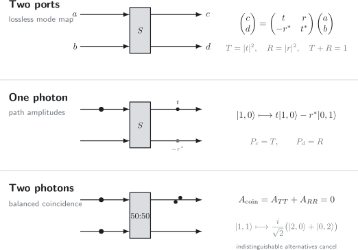
One lossless two-port unitary acts at several levels. It mixes mode operators and classical amplitudes, creates a path superposition from one input photon, and cancels the two indistinguishable coincidence amplitudes for one photon in each input of a balanced splitter. Port phases depend on convention; the probabilities and the cancellation do not.

State Transformations

Vacuum

The two-mode vacuum is invariant:

$$\hat U_{\mathrm{BS}}|0,0\rangle = |0,0\rangle.$$

A passive unitary cannot create excitations from vacuum. This separates beam splitters from squeezers and parametric amplifiers.

Coherent inputs

For coherent input amplitudes $\alpha$ and $\beta$, the output remains a product of coherent states:

$$|\alpha\rangle_a|\beta\rangle_b \longmapsto |t\alpha+r\beta\rangle_c |-r^*\alpha+t^*\beta\rangle_d.$$

The amplitudes obey the same matrix equation as classical complex fields. Ideal passive linear optics therefore does not entangle product coherent states. The detailed derivation, dark-port interference, and attenuation limit belong to Coherent Light.

Number in one input

For $n$ photons in port $a$ and vacuum in port $b$,

$$|n,0\rangle = \frac{ (\hat a^\dagger)^n }{ \sqrt{n!} } |0,0\rangle.$$

The output is

$$\begin{aligned} \hat U_{\mathrm{BS}}|n,0\rangle ={}& \sum_{k=0}^{n} \sqrt{\binom nk}\, t^k \\ &\quad\times (-r^*)^{n-k} |k,n-k\rangle. \end{aligned}$$

Consequently,

$$P(k,n-k) = \binom nk T^kR^{n-k}.$$

The port counts have a binomial distribution, but this does not mean that each photon carried a pre-existing independent path label. The state is a coherent superposition of occupation alternatives. Measurements diagonal in the output number basis reproduce the same binomial probabilities that an independent-trial story would predict for this particular input.

The moments are

$$\langle n_c\rangle=nT, \qquad \operatorname{Var}(n_c)=nTR,$$

with perfect number anticorrelation

$$n_c+n_d=n.$$

Gaussian moments

Passive linear optics also transforms Gaussian first and second moments. With the quadratures ordered as

$$\boldsymbol\xi = (X_1,\ldots,X_m,P_1,\ldots,P_m)^{\mathsf T},$$

a mode unitary $S$ induces the real matrix

$$O(S) = \begin{pmatrix} \operatorname{Re}S&-\operatorname{Im}S\\ \operatorname{Im}S&\operatorname{Re}S \end{pmatrix}.$$

It is both orthogonal and symplectic:

$$O^{\mathsf T}O=I, \qquad O\Omega O^{\mathsf T}=\Omega.$$

First moments and covariance matrices transform as

$$\overline{\boldsymbol\xi}_{\mathrm{out}} = O\overline{\boldsymbol\xi}_{\mathrm{in}}, \qquad V_{\mathrm{out}} = OV_{\mathrm{in}}O^{\mathsf T}.$$

This is the phase-space form of passive mode mixing. Gaussian States and Wigner Functions develops the covariance formalism; Squeezed Light explains how a beam splitter can redistribute squeezing and generate mode entanglement from suitable nonclassical inputs.

Single-Photon Interference

One occupied input

For one photon in port $a$,

$$|1,0\rangle \longmapsto t|1,0\rangle - r^*|0,1\rangle.$$

The click probabilities at ideal output detectors are

$$P_c=T, \qquad P_d=R.$$

For the symmetric balanced convention $t=1/\sqrt2$ and $r=i/\sqrt2$,

$$|1,0\rangle \longmapsto \frac{ |1,0\rangle+i|0,1\rangle }{ \sqrt2 }.$$

This is a coherent path superposition. A single beam splitter followed immediately by separate number measurements does not produce a phase-dependent fringe: the output alternatives are orthogonal and are counted separately. A fringe appears when alternatives are recombined or when the input already contains coherent amplitudes in both ports.

Two input amplitudes

Consider a general state in the one-photon sector,

$$\begin{gathered} |\psi_{\mathrm{in}}\rangle = \alpha|1,0\rangle + \beta|0,1\rangle, \\ |\alpha|^2+|\beta|^2=1. \end{gathered}$$

The output amplitudes obey

$$\begin{pmatrix} \alpha_c\\ \alpha_d \end{pmatrix} = \begin{pmatrix} t&r\\ -r^*&t^* \end{pmatrix} \begin{pmatrix} \alpha\\ \beta \end{pmatrix}.$$

Therefore

$$\begin{aligned} P_c &= T|\alpha|^2 + R|\beta|^2 \\ &\quad+ 2\operatorname{Re} \left( t r^* \alpha\beta^* \right). \end{aligned}$$

The last term is the one-photon interference term. It exists because two indistinguishable alternatives reach the same final detector: enter through $a$ and transmit, or enter through $b$ and reflect. Changing a relative input phase can route all probability to one output of a balanced splitter.

Does the output contain entanglement?

Relative to the output-mode tensor product, the state

$$\frac{ |1\rangle_c|0\rangle_d + e^{i\chi} |0\rangle_c|1\rangle_d }{ \sqrt2 }$$

is mode entangled. This statement is meaningful only after the subsystems have been declared as modes $c$ and $d$. It is not entanglement between two photons, because the state contains one photon. Questions about locality, accessible operations, vacuum reference phases, and particle-versus-mode language belong to Entanglement in Quantum Optics.

Hong–Ou–Mandel Interference

Ideal two-photon input

Place one photon in each input:

$$|1,1\rangle = \hat a^\dagger \hat b^\dagger |0,0\rangle.$$

Using the Schrödinger creation-operator map gives

$$\begin{aligned} \hat U_{\mathrm{BS}}|1,1\rangle ={}& \sqrt2\,tr\,|2,0\rangle \\ &+ (T-R)|1,1\rangle \\ &- \sqrt2\,r^*t^*\,|0,2\rangle. \end{aligned}$$

At a balanced splitter, $T=R$, so the coincidence amplitude vanishes. In the symmetric convention,

$$|1,1\rangle \longmapsto \frac{i}{\sqrt2} \left( |2,0\rangle + |0,2\rangle \right).$$

The overall factor $i$ has no effect on any probability. Both photons leave the same output, with equal probabilities for the two ports.

Which amplitudes cancel?

A coincidence can arise by two indistinguishable histories:

• both photons transmit;
• both photons reflect.

For a balanced lossless splitter, their amplitudes have equal magnitude and opposite phase. The labels “photon 1” and “photon 2” do not survive as physical particle identities. The detector sees one photon in each output, and the two assignments of identical bosons to that outcome must be added at the amplitude level.

The cancellation is a two-photon, fourth-order interference effect. It does not mean that photons attract, collide inside the optic, or choose the same port in advance.

Wave-packet overlap

Let

$$\begin{aligned} \hat a_f^\dagger &= \int d\omega\, f(\omega) \hat a^\dagger(\omega), \\ \int d\omega\, |f(\omega)|^2 &= 1, \end{aligned}$$

and define $\hat b_g^\dagger$ similarly. Their internal-mode overlap is

$$\mu = \langle f|g\rangle = \int d\omega\, f^*(\omega)g(\omega).$$

For ideal detectors that do not resolve the internal mode, the probability of one photon in each output is

$$P_{\mathrm{coin}} = T^2+R^2 - 2TR|\mu|^2.$$

At balance,

$$P_{\mathrm{coin}} = \frac12 \left( 1-|\mu|^2 \right).$$

Thus

$$\begin{aligned} |\mu|^2=1 &\quad\Longrightarrow\quad P_{\mathrm{coin}}=0, \\ |\mu|^2=0 &\quad\Longrightarrow\quad P_{\mathrm{coin}}=\frac12. \end{aligned}$$

The ideal balanced-dip visibility, normalized to the distinguishable coincidence level, is

$$\mathcal V = \frac{ P_{\mathrm{dist}}-P_{\mathrm{ind}} }{ P_{\mathrm{dist}} } = |\mu|^2.$$

This equality assumes one pure photon in each input, a balanced splitter, stable rates, and an appropriate subtraction or inclusion policy for backgrounds.

Delay scan

If one wave packet is delayed by $\tau$,

$$g(\omega) \longrightarrow g(\omega)e^{-i\omega\tau},$$

and

$$\mu(\tau) = \int d\omega\, f^*(\omega)g(\omega)e^{-i\omega\tau}.$$

A coincidence scan measures $|\mu(\tau)|^2$ under the ideal assumptions above. Its width is set by the mutual temporal coherence of the photon wave packets, not directly by detector timing resolution when the coincidence window is broad enough to collect each pair.

Mixed and correlated photons

For independent single-photon internal states $\rho_a$ and $\rho_b$, the balanced result generalizes to

$$P_{\mathrm{coin}} = \frac12 \left[ 1- \operatorname{Tr} \left( \rho_a\rho_b \right) \right].$$

The overlap $\operatorname{Tr}(\rho_a\rho_b)$ combines mismatch and mixedness. If the photons are entangled with unobserved partners or other degrees of freedom, their reduced states may be mixed even when average spectra look identical. A Hong–Ou–Mandel dip is therefore a powerful overlap diagnostic, but its visibility is not by itself a complete state tomography.

Indistinguishability is the canonical home for the general identical-particle principle. Photon Number States explains why low multiphoton contamination, high purity, and high indistinguishability are separate source properties.

Nonideal Beam Splitters

Imbalance

Even with perfectly identical photons,

$$P_{\mathrm{coin}}^{\mathrm{identical}} = (T-R)^2.$$

An unbalanced device cannot produce a zero coincidence probability. For fully distinguishable photons,

$$P_{\mathrm{coin}}^{\mathrm{dist}} = T^2+R^2.$$

The correct reference level must therefore use the measured $T$ and $R$ rather than assume one half.

Loss requires environmental modes

A two-by-two matrix for the accessible ports of a lossy component is subunitary. If one wrote only

$$\hat{\boldsymbol a}_{\mathrm{out}} = K \hat{\boldsymbol a}_{\mathrm{in}}, \qquad KK^\dagger<I,$$

then the output commutators would be too small. Quantum mechanics restores them by adding environmental operators:

$$\hat{\boldsymbol a}_{\mathrm{out}} = K \hat{\boldsymbol a}_{\mathrm{in}} + L \hat{\boldsymbol e}_{\mathrm{in}},$$

with

$$KK^\dagger+LL^\dagger=I.$$

The full transformation on system plus environment is unitary. Tracing over the inaccessible outputs produces a quantum channel. Loss before the splitter changes the input state; loss after it changes detection probabilities; unequal loss in the two arms can also reveal path information. These cases should not be folded into one unexplained efficiency number.

Spectral and polarization dependence

For wave packets, use

$$\begin{pmatrix} \hat c(\omega)\\ \hat d(\omega) \end{pmatrix} = S(\omega) \begin{pmatrix} \hat a(\omega)\\ \hat b(\omega) \end{pmatrix}.$$

Frequency-dependent splitting ratios and phases reshape the packets and can reduce interference even when the incident modes were identical. The same warning applies to polarization-dependent coatings and birefringent couplers. A scalar overlap measured before the device is insufficient if the device transforms the two inputs differently.

Detector and source effects

Raw coincidence contrast can be reduced by:

• multiphoton emission or more than one pair in a gate;
• uncorrelated background and detector dark counts;
• detector dead time, afterpulsing, saturation, or cross-talk;
• a coincidence window that excludes part of the wave packet or admits excess accidentals;
• timing drift and unstable input flux;
• unequal collection efficiencies;
• unresolved spectral, temporal, spatial, or polarization mismatch.

Threshold detectors are sufficient to observe a low-brightness Hong–Ou–Mandel dip, but the inference from clicks to an input overlap still requires a source and detector model. Reporting only a fitted visibility without its reference level, uncertainty, and background policy is incomplete.

What Beam Splitters Enable

Attenuation and channels

Mixing a signal with vacuum and discarding one output realizes the dilation of a pure-loss channel:

$$\hat c = \sqrt\eta\,\hat a + \sqrt{1-\eta}\,\hat e.$$

This model underlies propagation loss and detector inefficiency. The environmental output carries the information lost from the accessible signal.

Homodyne and displacement operations

A balanced beam splitter combines a signal with a strong local oscillator. Subtracting the two output photocurrents isolates a phase-selected field quadrature. Homodyne Detection owns the detector model and conditional record.

Mixing with a strong coherent auxiliary on a highly transmissive splitter approximates a displacement. Phase-Space Distributions explains how displacement followed by parity or counting samples optical quasidistributions.

Interferometers and networks

Beam splitters and phase shifters form arbitrary finite passive unitary networks. An $m$-mode unitary can be decomposed into a sequence of two-mode rotations and port phases. This is the foundation of multiport interferometers, linear-optical state preparation, boson sampling, and many photonic quantum-information protocols.

The existence of a unitary network does not imply deterministic interaction between photons. Passive linear optics acts linearly on modes; effective nonlinear gates generally need ancillary states, measurement, feedforward, postselection, or matter-mediated interactions.

Modeling Workflow

For a two-port calculation

1. Declare the complete input and output mode functions.
2. State $S$, including the reflection phases and whether it acts on annihilation operators.
3. Check unitarity or add environmental modes for loss.
4. Express the input using creation operators.
5. Apply the inverse creation-operator map to obtain the output state.
6. Trace over unresolved degrees of freedom.
7. Apply the detector POVM, efficiencies, and coincidence window.
8. Compare with a reference level computed using the same imbalance and detector model.

For an experiment report

Record at least:

• measured $T(\omega)$ and $R(\omega)$ over the occupied bandwidth;
• polarization and spatial-mode conventions;
• phase stability when amplitudes from both inputs interfere;
• source brightness, multiphoton contamination, and heralding condition;
• detector efficiency, timing response, dark counts, and dead time;
• raw and corrected data, including the correction model;
• the distinguishable reference and uncertainty used for visibility.

These details separate a reproducible mode-overlap measurement from a decorative dip.

Common Mistakes

• Treating a geometric port as a single normalized optical mode.
• Calling $T$ and $R$ amplitudes rather than intensity probabilities.
• Applying the same matrix to Heisenberg operators and Schrödinger creation operators without inversion or conjugation.
• Combining a state transformation from one phase convention with propagation phases from another.
• Assuming every reflection contributes $i$ without specifying reference planes and port labels.
• Claiming a single isolated splitter produces a phase fringe from one occupied input.
• Treating the binomial output of $|n,0\rangle$ as proof that photons carried independent hidden path labels.
• Describing Hong–Ou–Mandel bunching as attraction or collision.
• Calling a reduced dip uniquely evidence of temporal mismatch while ignoring spectrum, polarization, spatial mode, mixedness, and background.
• Using the balanced formula when the measured device is imbalanced.
• Representing loss with a subunitary operator map but omitting the environmental noise needed to preserve commutators.
• Inferring source purity from Hong–Ou–Mandel visibility alone.
• Calling every single-photon path superposition “two-particle entanglement.”
• Forgetting that frequency-dependent scattering can reshape broadband modes.

Connections

• Photonic Qubits assembles passive mode unitaries into encoded operations, Bell analyzers, resource preparation, and fusion networks while retaining explicit loss budgets.
• Quantum Optics supplies the chapter-wide state–transformation–measurement map.
• Quantized Electromagnetic Modes fixes the oscillator and continuum normalization behind each port.
• Photon Number States owns optical number statistics, source quality, and antibunching.
• Coherent Light develops coherent products under passive mixing, dark ports, and pure loss.
• Squeezed Light develops quadrature mixing and entanglement generated from squeezed inputs.
• Phase-Space Distributions connects passive mode transformations to quasidistributions and displaced measurements.
• Hanbury Brown–Twiss Interferometry shows why splitting one field routes, rather than creates, its normalized intensity correlation.
• AMO Experiment Index compares the Hong–Ou–Mandel coincidence record with HBT correlations and other landmark AMO observables.
• Interferometers composes beam splitters with arm phases to develop Mach–Zehnder statistics, shot noise, and squeezed phase readout.
• Entanglement in Quantum Optics owns path-mode entanglement and resource interpretation.
• Indistinguishability develops the general identical-particle origin of exchange interference.
• Gaussian States and Wigner Functions supplies the covariance-matrix description of passive Gaussian unitaries.
• Gaussian Channels develops loss and thermal-noise channels after environmental modes are traced out.
• Homodyne Detection owns balanced photocurrent subtraction and conditional quadrature records.

Exercises

1. Commutators force unitarity

Let

$$\hat c=t\hat a+r\hat b, \qquad \hat d=u\hat a+v\hat b.$$

Derive the conditions on $t,r,u,v$ required for $\hat c$ and $\hat d$ to be canonical independent bosonic modes. Show that the coefficient matrix is unitary.

Solution

The diagonal commutators give

$$\begin{aligned} [\hat c,\hat c^\dagger] &= |t|^2+|r|^2 =1, \\ [\hat d,\hat d^\dagger] &= |u|^2+|v|^2 =1. \end{aligned}$$

Independence requires

$$[\hat c,\hat d^\dagger] = tu^*+rv^* =0.$$

The remaining annihilation–annihilation commutators vanish automatically. If

$$S= \begin{pmatrix} t&r\\ u&v \end{pmatrix},$$

these three equations state that its two rows are orthonormal:

$$SS^\dagger=I.$$

Because $S$ is square, it follows that $S^\dagger S=I$ as well. Thus $S$ is unitary. Choosing $u=-r^*$ and $v=t^*$ gives the SU(2) convention used on this page.

2. Derive the mode rotation

Starting from

$$\hat U(\theta) = \exp\left[ \theta \left( e^{i\phi}\hat a^\dagger\hat b - e^{-i\phi}\hat a\hat b^\dagger \right) \right],$$

derive $\hat U^\dagger\hat a\hat U$ and $\hat U^\dagger\hat b\hat U$ by differential equations in $\theta$.

Solution

Define

$$\begin{aligned} \hat A(\theta) &= \hat U^\dagger(\theta) \hat a \hat U(\theta), \\ \hat B(\theta) &= \hat U^\dagger(\theta) \hat b \hat U(\theta). \end{aligned}$$

Let the anti-Hermitian generator be

$$\hat G = e^{i\phi}\hat a^\dagger\hat b - e^{-i\phi}\hat a\hat b^\dagger.$$

Differentiating gives

$$\frac{d\hat A}{d\theta} = \hat U^\dagger[\hat a,\hat G]\hat U = e^{i\phi}\hat B,$$

and

$$\frac{d\hat B}{d\theta} = \hat U^\dagger[\hat b,\hat G]\hat U = -e^{-i\phi}\hat A.$$

Therefore $d^2\hat A/d\theta^2=-\hat A$. With $\hat A(0)=\hat a$ and $d\hat A/d\theta|_0=e^{i\phi}\hat b$,

$$\hat A(\theta) = \hat a\cos\theta + e^{i\phi}\hat b\sin\theta.$$

Similarly,

$$\hat B(\theta) = \hat b\cos\theta - e^{-i\phi}\hat a\sin\theta.$$

The rotation preserves both canonical commutators and total photon number.

3. Rephase a balanced convention

Show explicitly that the symmetric matrix

$$S_i = \frac1{\sqrt2} \begin{pmatrix} 1&i\\ i&1 \end{pmatrix}$$

can be converted into the Hadamard matrix

$$S_H = \frac1{\sqrt2} \begin{pmatrix} 1&1\\ 1&-1 \end{pmatrix}$$

using only diagonal input and output phase matrices.

Solution

Choose

$$D_{\mathrm{in}} = \begin{pmatrix} 1&0\\ 0&i \end{pmatrix}, \qquad D_{\mathrm{out}} = \begin{pmatrix} 1&0\\ 0&-i \end{pmatrix}.$$

Then

$$D_{\mathrm{in}}^\dagger = \begin{pmatrix} 1&0\\ 0&-i \end{pmatrix}.$$

Direct multiplication gives

$$\begin{aligned} D_{\mathrm{out}} S_i D_{\mathrm{in}}^\dagger &= \frac1{\sqrt2} \begin{pmatrix} 1&i(-i)\\ (-i)i&(-i)(-i) \end{pmatrix} \\ &= \frac1{\sqrt2} \begin{pmatrix} 1&1\\ 1&-1 \end{pmatrix} =S_H. \end{aligned}$$

The two displayed matrices therefore differ only by port-coordinate phases. Any surrounding propagation and state phases must be rephased at the same time.

4. Binomial splitting of a number state

For input $|n,0\rangle$, derive the output number distribution and compute the mean, variance, and covariance of the two output counts.

Solution

The transformed state is

$$\hat U|n,0\rangle = \frac{ \left( t\hat a^\dagger-r^*\hat b^\dagger \right)^n }{ \sqrt{n!} } |0,0\rangle.$$

The binomial theorem and normalized Fock states give

$$\begin{aligned} \hat U|n,0\rangle ={}& \sum_{k=0}^{n} \sqrt{\binom nk}\, t^k \\ &\quad\times (-r^*)^{n-k} |k,n-k\rangle. \end{aligned}$$

Hence

$$P(n_c=k) = \binom nkT^kR^{n-k}.$$

The moments of a binomial variable are

$$\langle n_c\rangle=nT, \qquad \operatorname{Var}(n_c)=nTR.$$

Because $n_d=n-n_c$ in every outcome,

$$\langle n_d\rangle=nR, \qquad \operatorname{Var}(n_d)=nTR,$$

and

$$\operatorname{Cov}(n_c,n_d) = -\operatorname{Var}(n_c) = -nTR.$$

The negative covariance expresses exact conservation of the total input number.

5. Deterministic single-photon routing

Use the symmetric balanced convention

$$S_i = \frac1{\sqrt2} \begin{pmatrix} 1&i\\ i&1 \end{pmatrix}.$$

Find the relative phase $\chi$ in

$$|\psi_{\mathrm{in}}\rangle = \frac{ |1,0\rangle + e^{i\chi}|0,1\rangle }{ \sqrt2 }$$

that sends the photon entirely to output $c$, and the phase that sends it entirely to output $d$.

Solution

The output amplitudes are

$$\begin{aligned} \alpha_c &= \frac{ 1+i e^{i\chi} }{2}, \\ \alpha_d &= \frac{ i+e^{i\chi} }{2}. \end{aligned}$$

To make output $d$ dark, require

$$i+e^{i\chi}=0,$$

so $e^{i\chi}=-i$ and

$$\chi=-\frac{\pi}{2} \pmod{2\pi}.$$

Then $\alpha_c=1$. To make output $c$ dark, require

$$1+i e^{i\chi}=0,$$

so $e^{i\chi}=i$ and

$$\chi=\frac{\pi}{2} \pmod{2\pi}.$$

Then $\alpha_d=i$, whose phase is irrelevant to the unit detection probability. The routing is interference between the two input alternatives, not a change in the splitter’s $T$ or $R$.

6. Hong–Ou–Mandel interference away from balance

For one identical photon in each input, derive the coincidence probability for arbitrary $T$ and $R$. Compare it with the distinguishable value and find the visibility

$$\mathcal V = \frac{ P_{\mathrm{dist}}-P_{\mathrm{ind}} }{ P_{\mathrm{dist}} }.$$

Solution

The coefficient of $|1,1\rangle$ in the identical-photon output state is $T-R$. Therefore

$$P_{\mathrm{ind}} =(T-R)^2.$$

For distinguishable photons, the alternatives “both transmit” and “both reflect” add as probabilities:

$$P_{\mathrm{dist}} = T^2+R^2.$$

Their difference is

$$\begin{aligned} P_{\mathrm{dist}}-P_{\mathrm{ind}} &= T^2+R^2-(T-R)^2 \\ &= 2TR. \end{aligned}$$

Thus

$$\mathcal V = \frac{2TR}{T^2+R^2}.$$

It reaches one only at $T=R=1/2$. A nonzero minimum at zero delay can be caused by splitter imbalance even for perfectly overlapping photons.

7. Gaussian Hong–Ou–Mandel dip

Two photons have identical Gaussian spectral intensity

$$|f(\omega)|^2 = \frac{ 1 }{ \sqrt{2\pi}\sigma } \exp\left[ -\frac{ (\omega-\omega_0)^2 }{ 2\sigma^2 } \right].$$

One photon is delayed by $\tau$. Find the ideal balanced coincidence probability.

Solution

The overlap is the Fourier transform of the spectral intensity:

$$\mu(\tau) = \int d\omega\, |f(\omega)|^2 e^{-i\omega\tau}.$$

The Gaussian transform gives

$$\mu(\tau) = e^{-i\omega_0\tau} e^{-\sigma^2\tau^2/2}.$$

Therefore

$$|\mu(\tau)|^2 = e^{-\sigma^2\tau^2}.$$

For a balanced splitter,

$$P_{\mathrm{coin}}(\tau) = \frac12 \left( 1-e^{-\sigma^2\tau^2} \right).$$

The carrier phase cancels from the probability. The dip reaches zero at $\tau=0$ and approaches $1/2$ for delays much longer than $1/\sigma$.

8. Why a lossy map needs noise

Suppose an attenuator is written incorrectly as

$$\hat c=\sqrt\eta\,\hat a, \qquad 0<\eta<1.$$

Show what goes wrong. Add the minimum vacuum environment needed to repair the commutator, and derive the reduced output of an input one-photon state.

Solution

The incomplete map gives

$$[\hat c,\hat c^\dagger] = \eta \neq1.$$

Introduce an independent environment mode $\hat e$:

$$\hat c = \sqrt\eta\,\hat a + e^{i\varphi} \sqrt{1-\eta}\,\hat e.$$

Then

$$\begin{aligned} [\hat c,\hat c^\dagger] &= \eta[\hat a,\hat a^\dagger] + (1-\eta)[\hat e,\hat e^\dagger] \\ &=1. \end{aligned}$$

With the environment initially in vacuum, a unitary dilation maps

$$\begin{aligned} |1\rangle_a|0\rangle_e \longmapsto{}& \sqrt\eta\,|1,0\rangle \\ &+ e^{i\chi} \sqrt{1-\eta}\,|0,1\rangle, \end{aligned}$$

where $\chi$ depends on convention. Tracing over the environment removes the coherence between orthogonal environment states:

$$\rho_{\mathrm{out}} = \eta|1\rangle\langle1| + (1-\eta)|0\rangle\langle0|.$$

Loss is therefore not a noncanonical rescaling of an isolated operator. It is unitary mode mixing followed by loss of access to an environmental output.

References

1. A. Zeilinger, “General Properties of Lossless Beam Splitters in Interferometry,” American Journal of Physics 49, 882–883 (1981), doi:10.1119/1.12387.
2. C. K. Hong, Z. Y. Ou, and L. Mandel, “Measurement of Subpicosecond Time Intervals between Two Photons by Interference,” Physical Review Letters 59, 2044–2046 (1987), doi:10.1103/PhysRevLett.59.2044.
3. R. A. Campos, B. E. A. Saleh, and M. C. Teich, “Quantum-Mechanical Lossless Beam Splitter: SU(2) Symmetry and Photon Statistics,” Physical Review A 40, 1371–1384 (1989), doi:10.1103/PhysRevA.40.1371.
4. M. Reck, A. Zeilinger, H. J. Bernstein, and P. Bertani, “Experimental Realization of Any Discrete Unitary Operator,” Physical Review Letters 73, 58–61 (1994), doi:10.1103/PhysRevLett.73.58.
5. U. Leonhardt, “Quantum Physics of Simple Optical Instruments,” Reports on Progress in Physics 66, 1207–1249 (2003), doi:10.1088/0034-4885/66/7/203; arXiv:quant-ph/0305007.
6. F. Bouchard, A. Sit, Y. Zhang, R. Fickler, F. M. Miatto, Y. Yao, F. Sciarrino, and E. Karimi, “Two-Photon Interference: The Hong–Ou–Mandel Effect,” Reports on Progress in Physics 84, 012402 (2021), doi:10.1088/1361-6633/abcd7a; arXiv:2006.09335.
7. L. Mandel and E. Wolf, Optical Coherence and Quantum Optics (Cambridge University Press, 1995), Chapters 12 and 22, doi:10.1017/CBO9781139644105.
8. R. Loudon, The Quantum Theory of Light, 3rd ed. (Oxford University Press, 2000), Chapters 6 and 9.
9. S. M. Barnett and P. M. Radmore, Methods in Theoretical Quantum Optics (Oxford University Press, 2002), Chapter 2, doi:10.1093/acprof:oso/9780198563617.001.0001.
10. D. F. Walls and G. J. Milburn, Quantum Optics, 2nd ed. (Springer, 2008), Chapters 2 and 5, doi:10.1007/978-3-540-28574-8.
11. C. C. Gerry and P. L. Knight, Introductory Quantum Optics (Cambridge University Press, 2005), Chapters 4 and 6, doi:10.1017/CBO9780511791239.
12. P. Kok, W. J. Munro, K. Nemoto, T. C. Ralph, J. P. Dowling, and G. J. Milburn, “Linear Optical Quantum Computing with Photonic Qubits,” Reviews of Modern Physics 79, 135–174 (2007), doi:10.1103/RevModPhys.79.135.