Photonic Qubits

Purpose and Canonical Scope

Photonic qubits encode a two-dimensional quantum system in selected modes of the electromagnetic field. A photon can carry information through a waveguide, optical fibre, free space, or an interferometric network with little thermal excitation at optical frequencies. Passive optics can transform modes precisely, and photodetectors can measure them rapidly. Those same photons are difficult to store and difficult to make interact deterministically. Scalable photonic processing is therefore an architecture of sources, interference, ancillary states, measurement, switching, delays, classical feed-forward, and loss management rather than a collection of direct two-photon gates.

This page is the canonical architecture-level guide to discrete-variable photonic qubits. It owns the connections among:

• polarization, path, time-bin, and related rail encodings;
• deterministic emitters and heralded pair sources;
• passive linear-optical mode transformations;
• two-photon interference and measurement-induced entangling operations;
• circuit, cluster-state, and fusion-based computation;
• loss, mode mismatch, multiphoton contamination, and detector response;
• synchronization, switching, delay, feed-forward, and integrated photonics;
• optical links, matter memories, modular processors, and network interfaces;
• component metrics, accepted-event rates, and fault-tolerant resource accounting.

It does not duplicate the underlying quantum optics. Quantized Electromagnetic Modes owns field quantization and mode operators. Photon Number States owns single-photon states, source statistics, and nonclassicality. Beam Splitters owns two-port unitaries, phase conventions, and Hong–Ou–Mandel interference. Parametric Down-Conversion owns pair-source physics, joint spectra, heralding, and multipair emission. Photon Counting owns detector POVMs, efficiency, dark counts, timing, dead time, and response tomography. Graph States owns the graph-state construction and stabilizers. Here those objects become a processor and network contract.

Continuous-variable optical modes, Gaussian cluster states, and optical Gottesman–Kitaev–Preskill encodings belong to Continuous-Variable Platforms and the Bosonic Qubits architecture page. They are mentioned only when the boundary prevents a misleading comparison.

Record component efficiencies, chip scales, sampling experiments, and network distances are date-sensitive. The current evidence assessment belongs in Quantum Optics Frontiers. This page emphasizes durable architecture and labels dated examples explicitly.

The Architecture Contract

A photonic qubit is not specified by saying that one photon is present. The architecture must implement a complete map

$$\begin{gathered} \text{logical instruction} \\ \downarrow \\ \text{source requests and mode labels} \\ \downarrow \\ \text{synchronization and optical routing} \\ \downarrow \\ \text{interference, fusion, and measurement} \\ \downarrow \\ \text{time tags and classical feed-forward} \\ \downarrow \\ \text{accepted output or declared erasure}. \end{gathered}$$

A complete platform description identifies at least these layers:

Layer	Required specification
carrier	spatial, temporal, spectral, polarization, and propagation modes
encoding	code subspace, vacuum and multiphoton sectors, phase convention
source	emission process, trigger or herald, brightness, purity, indistinguishability
preparation	filters, converters, switches, delays, mode matching, synchronization
transformation	interferometer, phase settings, active elements, loss and drift
entanglement	direct nonlinearity, ancilla-assisted gate, graph generation, or fusion
measurement	threshold or number-resolving detector, basis analyzer, timing and response
classical control	herald logic, route selection, feed-forward, Pauli frame, decoder
network	fibre or free-space link, wavelength conversion, memory, herald protocol
infrastructure	pumps, stabilization, packaging, cryogenics, electronics, calibration
reporting	reference planes, accepted events, postselection, uncertainty, wall-clock rate

Several counts must remain separate:

1. Optical modes are addressable field degrees of freedom.
2. Source attempts are clock cycles in which generation is requested.
3. Generated photons occupy declared source modes before extraction loss.
4. Delivered photons reach a declared processor reference plane.
5. Detected photons produce accepted detector outcomes.
6. Encoded photonic qubits satisfy a rail-occupation rule.
7. Resource-state qubits belong to a verified graph or cluster state.
8. Logical qubits are protected by a declared code and decoder.

A processor with thousands of optical modes need not contain thousands of simultaneously occupied qubits. A detector record containing many photons in a sampling experiment need not implement a universal qubit circuit. A high conditional fidelity need not imply a high accepted-event rate. These distinctions are architectural, not semantic caution tape.

Modes Come Before Qubits

A photon occupies a mode

A normalized wave-packet creation operator can be written schematically as

$$\begin{aligned} a_f^\dagger &= \int d\omega\, f(\omega)a^\dagger(\omega),\\ \int d\omega\,|f(\omega)|^2&=1. \end{aligned}$$

The label $f$ can include spatial profile, propagation direction, polarization, and other degrees of freedom in addition to frequency. The one-photon state is

$$\lvert1_f\rangle = a_f^\dagger\lvert\mathrm{vac}\rangle.$$

Two nominal photons interfere as required only to the extent that all unresolved degrees of freedom match. Arrival time, spectrum, polarization, spatial profile, chirp, and source history can carry which-source information. A logical rail label does not erase hidden distinguishability.

For two pure normalized modes $f$ and $g$, define

$$\mathcal M = |\langle f\vert g\rangle|^2, \qquad 0\le\mathcal M\le1.$$

For a balanced beam splitter with one ideal photon in each input and otherwise matched detection, the coincidence probability is

$$P_{\mathrm{coin}} = \frac{1-\mathcal M}{2}.$$

Real Hong–Ou–Mandel visibility can also be affected by multiphoton emission, background, detector timing, imbalance, and normalization conventions.

The physical Hilbert space is larger than a qubit

Two bosonic modes $a$ and $b$ have Fock basis $\lvert n_a,n_b\rangle$ with unbounded occupations. A dual-rail qubit uses only the one-photon sector:

$$\begin{aligned} \lvert0_L\rangle &=\lvert1,0\rangle_{ab}, \\ \lvert1_L\rangle &=\lvert0,1\rangle_{ab}. \end{aligned}$$

The vacuum $\lvert0,0\rangle$ is a loss state. States such as $\lvert2,0\rangle$, $\lvert1,1\rangle$, and $\lvert0,2\rangle$ are multiphoton sectors, not valid states of this one-photon qubit. A physical description must retain them whenever source or detector imperfections can populate or confuse them.

The code projector is

$$P_{\mathrm{rail}} = \lvert1,0\rangle\langle1,0\rvert + \lvert0,1\rangle\langle0,1\rvert.$$

Conditional tomography after projecting with $P_{\mathrm{rail}}$ characterizes the surviving qubit. Unconditional performance must also report $\operatorname{Tr}(P_{\mathrm{rail}}\rho)$.

Encoding Families

Polarization

Choose two orthogonal polarizations of one spatial and temporal mode:

$$\begin{aligned} \lvert0_L\rangle&=\lvert H\rangle, \\ \lvert1_L\rangle&=\lvert V\rangle. \end{aligned}$$

Wave plates, polarization rotators, and polarization beam splitters implement preparation and analysis. Polarization is compact in free space and natural for many emitters and entangled-pair sources. In fibre or integrated circuits, birefringence, polarization-mode dispersion, stress, and coupling can rotate or dephase the basis. Active polarization tracking or conversion to another encoding may be required.

Polarization is still a dual-mode encoding: the rails are two orthogonal polarization modes rather than two paths. Photon loss takes both logical basis states to the same vacuum sector.

Path or spatial dual rail

Choose two waveguides or interferometer arms:

$$\begin{aligned} \lvert0_L\rangle&=\lvert1\rangle_a\lvert0\rangle_b, \\ \lvert1_L\rangle&=\lvert0\rangle_a\lvert1\rangle_b. \end{aligned}$$

A tunable Mach–Zehnder interferometer can implement an arbitrary one-qubit unitary by combining mode mixers and phase shifts. Path encoding maps naturally onto integrated photonics and local interferometers, but doubles the number of guided modes per qubit and makes path-dependent loss and phase drift logical errors.

The state

$$\alpha\lvert1,0\rangle +\beta\lvert0,1\rangle$$

depends on a relative optical phase. Stabilization and calibration must preserve that phase through every splitter, crossing, heater, switch, and coupling interface.

Time bin

Choose nonoverlapping early and late wave packets in one propagation channel:

$$\begin{aligned} \lvert0_L\rangle&=\lvert E\rangle, \\ \lvert1_L\rangle&=\lvert L\rangle. \end{aligned}$$

An unbalanced interferometer prepares and analyzes their coherent superposition. Time-bin encoding can be robust against slowly varying polarization transformations in fibre and supports temporal multiplexing. It requires detector timing sufficient to resolve bins, stable interferometric phase, matched dispersion, and active switching or delay when arbitrary single-qubit operations and feed-forward are needed.

The time-bin spacing must exceed the wave-packet duration and relevant timing jitter while fitting within coherence and switching windows. Closely spaced bins increase rate but tighten detector and modulator requirements; widely spaced bins increase delay and memory overhead.

Frequency bins and single rail

Frequency-bin qubits use two spectral modes and electro-optic or nonlinear frequency mixing. They can exploit dense wavelength multiplexing, but require phase-coherent frequency processors and careful treatment of dispersion and spectral leakage.

A single-rail qubit uses

$$\lvert0_L\rangle=\lvert0\rangle, \qquad \lvert1_L\rangle=\lvert1\rangle$$

of one mode. It uses fewer rails, but a coherent superposition of vacuum and one photon requires a phase reference, and photon loss maps $\lvert1\rangle$ into the logical $\lvert0\rangle$ rather than an orthogonal flag. Dual rail is often preferred when located vacuum is operationally useful.

Encoding conversion is an operation

A network may convert path to polarization, polarization to time bin, or an emitter wavelength to the telecom band. Such conversion is not merely a change of notation. It has efficiency, noise, bandwidth, phase, and mode-overlap specifications. The conversion must preserve arbitrary superpositions, not only transmit the two basis states separately.

Source Layer

What an ideal source promises

For a triggered discrete-variable architecture, the ideal instruction is:

On each accepted clock cycle, deliver one photon into a declared normalized mode at a declared reference plane, with no vacuum or multiphoton component.

No source is summarized by one number. A useful source record includes:

Quantity	Operational question
generation probability	how often is the desired excitation created per request?
extraction and coupling	how often does it reach the output reference plane?
number purity	how much vacuum and multiphoton contamination remains?
spectral purity	is the heralded photon in one mode or a mixture?
indistinguishability	do photons from relevant times and sources interfere?
timing	what are emission jitter, pulse duration, and repetition rate?
stability	do frequency, brightness, and mode remain calibrated over time?
scalability	can many sources be tuned, pumped, and packaged simultaneously?

A small $g^{(2)}(0)$ constrains multiphoton statistics under a measurement model. It does not determine extraction efficiency, mutual indistinguishability, spectral purity, or accepted-photon rate.

Deterministic emitters

Quantum dots, atoms, ions, molecules, color centers, and other localized emitters can be excited so that one radiative transition produces at most one photon per cycle. A cavity or waveguide can enhance emission into a desired mode. Resonant excitation can improve coherence and reduce timing jitter.

The word deterministic should be attached to a reference plane. Exciting an emitter with near-unit probability is not the same as delivering a photon after branching, extraction, filtering, conversion, coupling, switching, and transport. Independent emitters must also be tuned into mutual spectral and temporal overlap without adding unacceptable noise.

Heralded pair sources

Spontaneous parametric down-conversion and spontaneous four-wave mixing produce correlated photon pairs. In a simple two-mode squeezed description,

$$\lvert\psi\rangle = \sqrt{1-\lambda^2} \sum_{n=0}^{\infty} \lambda^n\lvert n,n\rangle.$$

Detecting one mode heralds the likely presence of its partner. At low gain, vacuum dominates; increasing gain raises the pair rate and the probability of unwanted multiple pairs. Filtering can improve spectral purity while lowering brightness and heralding efficiency. Number-resolving herald detectors can reject some multipair events but do not undo loss before the detector.

The canonical source derivation and joint-spectral analysis belong in Parametric Down-Conversion. At architecture level, the key output is a calibrated conditional state and the unconditional probability that it reaches the processor.

Multiplexing

If $M$ independent source bins each succeed with probability $p$, the probability of at least one success is

$$P_{\ge1} = 1-(1-p)^M.$$

Multiplexing can turn heralded uncertainty into a higher delivery probability, but it consumes source modes, herald detectors, routing switches, delay, and classical decisions. If the selected route has transmissivity $\eta_{\mathrm{sw}}$, the useful probability is no larger than

$$P_{\mathrm{del}} \le \eta_{\mathrm{sw}} \left[1-(1-p)^M\right].$$

Correlated pumps, switch contention, multiple simultaneous successes, multipair noise, and finite feed-forward time require a fuller scheduler.

Passive Linear Optics

Mode transformations

For $m$ lossless optical modes, a passive interferometer acts by a unitary matrix $U$:

$$b_j^\dagger = \sum_{k=1}^{m} U_{jk}a_k^\dagger, \qquad U^\dagger U=I.$$

Beam splitters and phase shifters can synthesize any finite-dimensional passive mode unitary. The transformation conserves total photon number:

$$\sum_j b_j^\dagger b_j = \sum_k a_k^\dagger a_k.$$

In the one-photon sector of two rails, this gives arbitrary one-qubit rotations. Large interferometers can implement mode permutations, Fourier transforms, state analyzers, sampling networks, and the optical parts of entangling measurements.

Real devices require an enlarged scattering matrix that includes loss ports. The implemented transfer matrix can depend on wavelength, polarization, temperature, drive history, and fabrication variation. A target unitary fidelity alone does not report insertion loss.

Why two-qubit gates are difficult

Passive linear optics transforms field modes linearly. It does not provide a deterministic interaction energy conditioned on two separate photons being present. Two identical photons can interfere, but interference alone does not make every desired dual-rail two-qubit unitary deterministic.

There are three broad responses:

1. use a strong optical or matter-mediated nonlinearity;
2. use ancillary photons, photodetection, and feed-forward to induce a measurement-conditioned gate;
3. avoid an online deterministic gate by preparing entangled resources and consuming them through measurements or fusions.

The Knill–Laflamme–Milburn result established that ideal single photons, passive optics, photodetection, ancillas, and feed-forward are sufficient for scalable universal quantum computation in principle. The effective nonlinearity comes from measurement and conditioning. Sufficiency does not mean low overhead: source probabilities, detector efficiencies, failed measurements, ancilla preparation, switching, and loss determine the architecture.

Bell-state analysis

For standard dual-rail qubits, passive linear optics without suitable ancillary resources cannot deterministically distinguish all four Bell states. The familiar analyzer identifies only a subset and succeeds with at most one half under its standard assumptions. Ancillary photons, additional modes, number resolution, nonlinearities, or hyperentanglement can raise the success probability, each with a resource cost.

This limitation matters because Bell measurements drive teleportation, entanglement swapping, the untrusted relay in measurement-device-independent QKD, and many fusion gates. A network claim should report both conditional Bell-state fidelity and unconditional successful-analysis probability.

Computational Architectures

Circuit-model linear-optical computation

Circuit-model schemes compile logical gates into:

• deterministic one-qubit interferometers;
• probabilistic entangling gadgets;
• offline ancillary states;
• photon counting;
• active feed-forward and routing.

If an entangling gadget succeeds with probability $p_g$, a circuit containing $G$ such gadgets would have naive direct success $p_g^G$. Scalable schemes do not simply postselect the whole circuit. They use teleportation, offline resource preparation, multiplexing, encoding, and error correction so that failed attempts become located events that can be retried or decoded.

The price shifts into resource-state factories and optical depth. A gate list without ancilla photons, source attempts, detectors, switches, delays, and accepted-event rate is not a complete circuit resource estimate.

Cluster-state and one-way computation

A graph state can be written

$$\lvert G\rangle = \prod_{\{i,j\}\in E} CZ_{ij} \lvert+\rangle^{\otimes |V|}.$$

Measurement-Based Quantum Computation prepares the entangled resource first and then consumes it as an ideal pattern. Single-qubit measurements then consume vertices and propagate the logical state through the graph. Measurement bases can depend on earlier outcomes, and random Pauli byproducts are corrected physically or tracked in a Pauli frame.

This moves entangling work offline and aligns with destructive photodetection. It does not make resource generation free. A large useful cluster must be built from sources and probabilistic optical operations with enough redundancy to survive failed fusions and photon loss. Graph States owns the state and stabilizer structure.

Fusion-based computation

Fusion-based quantum computation treats small entangled resource states and projective entangling measurements as the primitive operations. A fusion consumes photons from resource states and attempts to connect their encoded graphs. Success, known failure, loss, and detector faults are passed directly into a fault-tolerant decoding problem.

This is a better hardware match than pretending photons possess deterministic in-place two-qubit gates. A complete fusion specification includes:

• input resource-state graph and verification;
• optical analyzer and ancillary modes;
• ideal fusion success probability;
• loss locations and detector outcome alphabet;
• which failures are heralded;
• feed-forward and switching requirements;
• resulting graph transformation for every outcome;
• decoder and threshold model.

The often-quoted loss thresholds of a proposed fusion architecture are theoretical results under a declared resource state, noise model, fusion network, and decoder. They are not measured loss budgets for every photonic machine.

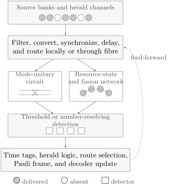
A discrete photonic processor is a synchronized flow rather than a static register. Sources and heralds establish which photons exist; conditioning and delays align their modes; interferometers enact one-qubit transformations or fusion measurements; detectors produce destructive outcomes; and classical logic selects routes, updates frames, and declares losses. A telecom interface can carry the same photonic encoding between modules when conversion and coupling are included in the loss budget.

Detection and Feed-Forward

Detection is usually destructive

Optical photon counting typically absorbs the photon. A terminal basis measurement is natural; a nondestructive mid-circuit measurement generally requires a matter interaction, teleportation, or a larger optical construction. Measurement-based and fusion architectures embrace this destruction by making measured photons disposable resource qubits.

Two detector classes recur:

• a threshold detector distinguishes no click from one-or-more clicks;
• a photon-number-resolving detector estimates the incident photon number over a declared mode and time gate.

Number resolution can distinguish valid one-photon outcomes from collisions or some multiphoton faults. It does not restore photons lost upstream.

For ideal number state $\lvert n\rangle$, detector efficiency $\eta_d$, and no dark count, the no-click probability of a threshold detector is

$$P(0\mid n) = (1-\eta_d)^n.$$

With independent dark-click probability $d$ per gate,

$$P(0\mid n) = (1-d)(1-\eta_d)^n.$$

The full response also includes background, recovery, jitter, saturation, and mode selectivity. The Photon Counting page owns that detector model.

Feed-forward has a physical path length

Suppose a detection outcome must control a later optical element. The photon being controlled must remain available while detection, electronics, and switching finish:

$$\tau_{\mathrm{delay}} \ge \tau_{\mathrm{det}} +\tau_{\mathrm{elec}} +\tau_{\mathrm{switch}} +\tau_{\mathrm{margin}}.$$

For group velocity $v_g$, the corresponding propagation length is

$$L_{\mathrm{delay}} = v_g\tau_{\mathrm{delay}}.$$

Nanosecond decisions can require metres of waveguide or fibre. Longer delay adds propagation loss, dispersion, footprint, phase drift, and scheduling constraints. Fast feed-forward is therefore an optical and electronic co-design problem.

Pauli frames reduce physical switching

When a measurement induces a known Pauli byproduct, software can often update the interpretation of later operations rather than applying an immediate physical correction. This Pauli-frame tracking reduces switch depth and loss. It does not remove adaptive changes of non-Clifford measurement bases or all routing decisions.

Loss and Error Budgets

Optical loss composes multiplicatively

If a photon traverses components with transmissivities $\eta_1,\ldots,\eta_K$, then

$$\eta_{\mathrm{path}} = \prod_{k=1}^{K}\eta_k.$$

In decibels,

$$\mathcal L_{\mathrm{dB}} = -10\log_{10}\eta_{\mathrm{path}},$$

so component losses add. Coupling, propagation, bends, crossings, filters, switches, delays, conversion, and detector inefficiency must all be assigned to explicit reference planes.

If $N$ required photons independently survive with probability $\eta$, the all-photon probability is

$$P_{\mathrm{all}}=\eta^N.$$

This exponential is why a conditional fidelity after detecting all photons can coexist with a poor unconditional rate.

Loss can be an erasure, but not always

For a dual-rail qubit known to contain one photon, loss produces the orthogonal vacuum state $\lvert0,0\rangle$. A complete terminal measurement with well-characterized detectors can label no click as an erasure. Inside a network, however, the absence may be discovered only later, and inefficient detectors or dark counts can confuse loss with measurement outcomes.

The useful record includes:

• probability of loss;
• probability that loss is flagged;
• spatial and temporal resolution of the flag;
• false-erasure and missed-erasure rates;
• operations attempted after the unknown loss time;
• correlations from common coupling or switching failures.

Erasure and Loss Channels owns the channel-level distinction among flagged erasure, unflagged loss, postselected survival, and bosonic attenuation.

Mode mismatch is a coherent systems error

Imperfect overlap lowers two-photon interference and can entangle logical rails with unobserved spectral or temporal modes. If those modes are traced out, the logical state dephases or mixes. The error may vary with source pair, time separation, temperature, and route. Characterizing one adjacent-pulse Hong–Ou–Mandel dip does not establish long-term mutual indistinguishability across a source array.

Multiphoton contamination is not simple loss

A pair source can produce two pairs, and an imperfect emitter can re-excite. Threshold detectors may accept a multiphoton event as an ordinary click. The result can create false heralds, incorrect fusion outcomes, or unmodeled correlations. Number-resolving detectors and source monitoring help only under their calibrated efficiency and response.

Phase, polarization, and switching errors

Path and time-bin qubits depend on relative phase. Polarization qubits depend on controlled birefringence. Active switches and modulators can add insertion loss, finite extinction, ringing, thermal crosstalk, and time-dependent phase. These are logical errors even when no photon is lost.

Correlated faults

Photonic errors are not automatically independent. One pump fluctuation can affect many pair sources; one thermal phase shifter can drift neighboring interferometers; one fibre connector can remove both rails; detector crosstalk can correlate outcomes; a clock error can shift an entire time-bin frame. Fault-tolerance analyses need measurements of these shared causes.

Network Compatibility

Flying qubits are a native strength

Photonic qubits can leave a processor without a separate quantum transducer when their wavelength and encoding already match the transmission channel. Telecom-band photons are compatible with low-loss standard fibre; visible or near-infrared emitters may require quantum frequency conversion. Interconnects and Transduction owns the full source-to-target link contract and the converter metrics used when the carrier, frequency band, or encoding changes.

For fibre attenuation $\alpha$ in decibels per unit length and distance $L$,

$$\eta_{\mathrm{fib}}(L) = 10^{-\alpha L/10}.$$

Direct transmission therefore decreases exponentially with distance. A repeater architecture uses heralded elementary links, memories, and entanglement swapping to change end-to-end rate scaling. It does not violate loss; it distributes attempts across segments and waits for successful links.

Encoding choice changes channel engineering

Encoding	Network advantage	Network burden
polarization	simple analyzers and free-space interfaces	fibre birefringence and polarization tracking
time bin	robust to slow polarization drift	unbalanced interferometers, timing and dispersion
frequency bin	wavelength multiplexing and routing	coherent frequency conversion and spectral phase
path	natural on chip	two physical channels and path-phase stability off chip

Conversion between a chip’s path encoding and a fibre’s polarization or time-bin encoding can be useful, but the converter’s efficiency and process fidelity must both be measured.

Matter memories change the timing contract

Matter qubits can store entanglement while photons attempt remote links. A useful elementary-link condition is not merely long memory coherence; the memory should outlast the stochastic waiting and communication time:

$$T_{\mathrm{mem}} \gg \frac{1}{R_{\mathrm{link}}} +\tau_{\mathrm{classical}}.$$

The link rate depends on emission, collection, conversion, transmission, interference, detector, and herald acceptance. If two remote photons must both arrive at a central station, several efficiencies enter quadratically.

Network-compatible does not mean network-complete

A high-fidelity chip-to-chip channel conditional on arrival establishes state preservation for surviving photons. A useful modular computer additionally needs low loss, synchronized sources, entangling protocols, memories or buffers, feed-forward, and a code that tolerates failed links. A QKD network distributes secret classical keys; it is not automatically a network of coherent quantum processors.

Infrastructure and Integration

Free-space, fibre, and integrated optics

Free-space optics offers flexible access and rapid prototyping. Fibre offers low-loss guided transmission and mature connectors. Integrated photonics offers dense, stable interferometers, repeatable lithography, and electrical control. Large systems often combine all three.

Integration changes the error budget rather than deleting it. Relevant constraints include:

• propagation loss and sidewall scattering;
• fibre-to-chip and chip-to-chip coupling;
• waveguide crossings, bends, and polarization handling;
• fabrication variation in splitters, resonators, and sources;
• thermal or electro-optic tuning power;
• optical pump rejection near single-photon detectors;
• superconducting detector temperature and cryogenic wiring;
• yield, screening, packaging, repair, and calibration at wafer scale.

Calling an optical qubit room-temperature hardware because it propagates at room temperature can be misleading. Sources, memories, frequency converters, and high-efficiency superconducting detectors may require cryogenic systems.

Calibration is a mode graph

An interferometer mesh has many coupled phases and losses. Calibrating each phase shifter separately may fail when thermal crosstalk or shared electrical drivers are active. Sources must be calibrated against filters and detector gates; detectors against arrival-time and wavelength distributions; switches against the routes they actually serve.

A useful digital twin contains:

• a complex transfer matrix versus wavelength and control settings;
• source density matrices or mode-overlap models;
• component and path transmissivities;
• detector response matrices and timing kernels;
• drift and crosstalk dependencies;
• uncertainty and validation data outside the calibration set.

Synchronization is a first-class resource

Independent photons must meet within their coherence time. Clock distribution, pump timing, emitter jitter, path delay, dispersion, and detector time tags all contribute. Temporal multiplexing increases mode count but also increases the scheduler’s responsibility to track which bins contain valid resources.

Throughput and Resource Accounting

Accepted-event rate

Let the clock rate be $f_{\mathrm{rep}}$ and the probability that a complete trial is accepted be $p_{\mathrm{acc}}$. Then

$$R_{\mathrm{acc}} = f_{\mathrm{rep}}p_{\mathrm{acc}}.$$

For a simple $N$-photon event,

$$p_{\mathrm{acc}} \sim \left( p_{\mathrm{src}}\eta_{\mathrm{path}}\eta_d \right)^N p_{\mathrm{logic}},$$

where $p_{\mathrm{logic}}$ contains the success probabilities of required fusions, heralds, and acceptance tests. This factorization is only a baseline: source correlations, multiplexing, detector saturation, and route contention can alter it.

Conditional fidelity $F_{\mathrm{cond}}$ and $R_{\mathrm{acc}}$ answer different questions. Multiplying them does not generally produce a universal utility metric. Report both, together with output distribution, uncertainty, and the task’s success criterion.

Resource factories

Cluster and fusion architectures continuously consume small entangled states. A useful factory metric is not only resource-state fidelity but the rate at which verified states reach the fusion network:

$$R_{\mathrm{res}} = f_{\mathrm{rep}} p_{\mathrm{gen}} p_{\mathrm{verify}} \eta_{\mathrm{deliver}}.$$

The system must balance factory rate, buffer depth, fusion demand, detector recovery, and decoder latency. Overproduction wastes photons and detector bandwidth; underproduction stalls the logical clock.

Postselection changes the task

Discarding every shot with missing photons can be valid for a proof-of- principle conditional experiment. It is not a scalable strategy when $p_{\mathrm{acc}}$ falls exponentially. A performance claim should state:

• all event filters and their order;
• accepted and total attempts;
• whether filters use information unavailable in real time;
• conditional output quality;
• unconditional success probability and wall-clock rate;
• whether the intended application permits postselection.

Boson-sampling experiments, heralded gates, communication links, and fault-tolerant logical computation have different acceptance contracts.

Fault-Tolerant Fit

Architectural opportunities

Photonic systems offer several fault-tolerance-relevant features:

• passive mode transformations can have low coherent noise;
• photons couple weakly to thermal environments during propagation;
• loss often leaves a dual-rail code space and can become a located erasure;
• destructive measurements are fast and natural;
• resource states can be prepared and verified offline;
• multiplexing can convert probabilistic preparation into heralded supply;
• optical links naturally connect modules;
• fabrication can replicate many interferometric components.

Architectural pressures

The same platform faces unusual costs:

• photonic qubits are not naturally stationary;
• every delay or switch adds loss;
• source and detector probabilities compound across many photons;
• deterministic photon–photon gates are not supplied by passive optics;
• most syndrome information is generated through destructive measurement;
• errors in hidden modes can evade a rail-only model;
• resource factories and detectors may dominate component count and power;
• decoder and route decisions must keep pace with flying time bins.

Loss-aware codes and cluster redundancy

Tree clusters, parity encodings, topological cluster states, and fusion networks can tolerate heralded failures and loss under specified thresholds. The code must know enough about where and when a photon disappeared. Loss that is mistaken for a valid detector outcome is more damaging than a clean erasure.

Threshold claims are not portable constants. They depend on:

• source and resource-state model;
• per-component and per-photon loss placement;
• fusion analyzer and success probability;
• detector number resolution and dark events;
• depolarizing, dephasing, and distinguishability errors;
• correlations;
• decoder and lattice geometry;
• overhead target and logical circuit.

What would establish scalable fault tolerance

Strong evidence would combine:

1. continuously supplied verified resource states;
2. repeated encoded operations or measurements;
3. real-time loss and outcome processing;
4. logical error suppression as code resources increase;
5. accepted-event and wall-clock rates;
6. operation under the full parallel source, switch, and detector load;
7. an end-to-end resource ledger including cryogenic and classical systems.

No general-purpose fault-tolerant photonic quantum computer satisfying that complete contract had been demonstrated by August 2026.

Dated Evidence Through August 2026

The following milestones answer different questions and should not be ranked by one number.

Date	Demonstrated or established object	What it supports	What it does not establish
2001	Knill–Laflamme–Milburn construction	ideal linear optics, photons, detectors, ancillas, and feed-forward are computationally universal	practical overhead or fault-tolerant component performance
2005	four-photon one-way cluster-state experiment	measurement-based photonic primitives can be implemented	scalable resource generation or loss tolerance
2010s	integrated interferometers, bright emitters, and high-efficiency detectors	key components can achieve high quality in controlled tests	simultaneous system-scale yield and accepted rate
2022	216-mode programmable Gaussian boson-sampling processor	large temporally multiplexed photonic sampling and dynamic interferometry	discrete-qubit universal computation or fault tolerance
2023	fusion-based fault-tolerance construction	small resource states and fusion measurements form a hardware-aligned computational model with explicit loss thresholds	a measured machine operating at that threshold
2024	remote matter memories entangled through telecom fibre	photons can link stored qubits through conversion, transmission, interference, and heralding	a multi-link repeater beating direct transmission
2025	co-integrated silicon-photonic source, filters, interferometers, detectors, fusion, and chip link	a manufacturable component stack can combine major discrete-photonic functions	an end-to-end fault-tolerant computer or loss-independent performance

The 2025 integrated-platform paper reported $99.98\%\pm0.01\%$ dual-rail state-preparation-and-measurement fidelity, $99.50\%\pm0.25\%$ independent-source interference visibility, $99.22\%\pm0.12\%$ fusion fidelity, and $99.72\%\pm0.04\%$ chip-link fidelity. Those values were conditional on photon detection and explicitly excluded loss; the sources were heralded and nondeterministic. The appropriate conclusion is that a high-quality integrated component stack was demonstrated. Combining the best component values into a projected large machine remains an engineering and fault-tolerance model, not a measured end-to-end benchmark.

Quantum Optics Frontiers maintains the broader dated evidence for sources, detectors, discrete and continuous architectures, sampling, integrated photonics, memories, and networks.

Advantages and Bottlenecks

Durable advantages

1. Propagation. Optical photons are natural flying qubits for chip, fibre, and free-space links.
2. Low thermal occupation. Optical-frequency modes have negligible equilibrium thermal population in ordinary environments.
3. Precise passive control. Interferometers implement stable, high-quality mode transformations.
4. Fast destructive measurement. Photon counting naturally supplies projective outcomes, heralds, and time tags.
5. Multiplexing. Path, time, frequency, and polarization provide many addressable modes.
6. Offline resources. Probabilistic states can be generated and verified before touching data.
7. Network compatibility. The computational carrier can also be the communication carrier.
8. Manufacturing base. Integrated photonics can draw on mature semiconductor and telecommunications processes.

Persistent bottlenecks

1. Loss. Source, coupling, switching, delay, routing, conversion, and detection efficiencies multiply.
2. Source simultaneity. Many mutually indistinguishable photons must be delivered in the correct clock cycle.
3. No simple deterministic entangler. Passive optics requires measurement, ancillas, nonlinearities, or resource-state architectures.
4. Mode matching. Hidden temporal and spectral structure can spoil interference without changing a rail label.
5. Feed-forward delay. Classical decisions require physical optical storage and add loss.
6. Detector infrastructure. High efficiency and number resolution often require cryogenic detectors and substantial electronics.
7. Resource overhead. Factories, switches, delays, herald detectors, and discarded attempts can outnumber logical data resources.
8. Conditional reporting. Excellent surviving-event fidelity can obscure poor unconditional rate.
9. Integration tradeoffs. Dense fabrication couples optical loss, thermal tuning, pump rejection, detector yield, and packaging.

Worked Architecture Audit

Consider a notional six-photon fusion event clocked at $f_{\mathrm{rep}}=1\,\mathrm{MHz}$. Each source bank delivers its required photon with probability $p_{\mathrm{src}}=0.80$. Each photon then traverses twelve components of transmissivity $\eta_c=0.995$ and is measured by a detector with efficiency $\eta_d=0.95$. The event requires two independent fusions, each with ideal success probability $p_f=0.50$.

1. Propagation and detection

The single-photon path-and-detector efficiency is

$$\begin{aligned} \eta_1 &= \eta_c^{12}\eta_d \\ &= (0.995)^{12}(0.95) \\ &\approx0.895. \end{aligned}$$

All six delivered photons survive and register with probability

$$\eta_1^6 \approx (0.895)^6 \approx0.514.$$

2. Source simultaneity

All six sources deliver in the same cycle with probability

$$p_{\mathrm{src}}^6 =(0.80)^6 \approx0.262.$$

This factor would be absent from a fidelity reported only after six photons were detected.

3. Fusion acceptance

The two ideal fusions both succeed with probability

$$p_f^2 =(0.50)^2 =0.25.$$

Under the independent baseline, the accepted-event probability is

$$\begin{aligned} p_{\mathrm{acc}} &= p_{\mathrm{src}}^6 \eta_1^6 p_f^2 \\ &\approx (0.262)(0.514)(0.25) \\ &\approx0.0337. \end{aligned}$$

The idealized accepted rate is therefore

$$R_{\mathrm{acc}} \approx 3.37\times10^4\,\mathrm{s}^{-1}.$$

Dead time, route contention, false heralds, multiphoton rejection, resource verification, and decoder barriers would reduce it.

4. Feed-forward storage

Suppose detection, electronics, switching, and margin require $35\,\mathrm{ns}$, $20\,\mathrm{ns}$, $10\,\mathrm{ns}$, and $5\,\mathrm{ns}$ respectively. Then

$$\tau_{\mathrm{delay}} \ge 70\,\mathrm{ns}.$$

For $v_g=2.0\times10^8\,\mathrm{m\,s^{-1}}$,

$$L_{\mathrm{delay}} \ge 14\,\mathrm{m}.$$

This simple calculation explains why electronic latency becomes metres of fibre or waveguide and why feed-forward loss belongs in the architecture.

Audit conclusion

The component quality may be high while source simultaneity, all-photon survival, and fusion probability reduce acceptance to a few percent. The next questions are whether multiplexing raises $p_{\mathrm{src}}$ after switch loss, whether the 14-m delay preserves mode quality, whether detector outcomes identify loss, and whether error correction can consume the resulting event stream faster than resource factories replenish it.

Evidence and Reporting Ledger

Claim class	Minimum evidence
photonic qubit	complete mode labels, code projector, vacuum and multiphoton populations
source	reference plane, brightness, extraction, $g^{(2)}(0)$, purity, indistinguishability, stability
one-qubit operation	transfer matrix, insertion loss, wavelength dependence, drift, simultaneous context
two-photon interference	source pair, delay scan, raw and corrected visibility, multiphoton and detector model
fusion or gate	success probability, conditional process quality, loss, ancillas, outcome map, feed-forward
cluster resource	graph, preparation probability, loss map, stabilizers or witnesses, accepted rate
detector	efficiency, outcome resolution, dark counts, jitter, dead time, saturation, reference plane
link	encoding, wavelength, distance, attenuation, conversion, arrival probability, conditional channel quality
logical result	code, physical and logical resources, decoder, rounds, loss handling, scaling and throughput
integrated platform	die and wafer yield, active components, packaging, cryogenic load, calibration and uptime
advantage claim	task, distribution, validator, all losses and postselection, wall-clock rate, classical baseline

Common Mistakes

Saying that the photon is the qubit

The qubit is an encoding in a declared mode subspace. Polarization, path, time, frequency, vacuum, and multiphoton sectors must be specified.

Calling a weak coherent pulse a single photon

A weak coherent state contains vacuum and multiphoton terms. Attenuation reduces their means but does not project onto the one-photon sector.

Equating antibunching with complete source quality

Small $g^{(2)}(0)$ constrains multiphoton emission. It does not certify delivery probability, spectral purity, indistinguishability, or stability.

Treating Hong–Ou–Mandel visibility as a gate fidelity

Two-photon visibility probes mode overlap under a declared experiment. A gate also depends on interferometer settings, ancillas, loss, detector response, and outcome conditioning.

Saying linear optics cannot compute

Passive optics alone does not supply deterministic photon–photon interactions. Linear optics combined with nonclassical ancillas, measurement, and feed-forward can be universal in principle.

Calling a heralded source deterministic

A herald reveals that a probabilistic event likely occurred. Delivery still depends on pair generation, herald detection, routing, and output transmission.

Treating photon loss as always flagged

Dual-rail loss leaves the code space, but the architecture must actually detect absence at a useful location and time without confusing detector inefficiency or dark counts.

Reporting only conditional fidelity

The surviving state can have excellent fidelity while almost all trials are discarded. Report acceptance probability and wall-clock rate.

Equating a large mode count with a qubit count

Many optical modes may be vacuum, continuously variable, or part of a sampling network. State the occupied encoding and computational model.

Calling a Bell measurement deterministic

The success probability depends on encoding, analyzer, ancillary states, number resolution, and nonlinear resources. Standard passive dual-rail analysis is incomplete.

Assuming network compatibility makes a repeater

Propagation through fibre is one component. A repeater also needs heralded links, memories, swapping, control, rate analysis, and a direct-transmission comparison.

Calling integrated photonics room-temperature computing

The waveguides may operate near room temperature while emitters, memories, or high-efficiency superconducting detectors require cryogenic support.

Exercises

1. Identify the code and leakage sectors

For two path modes $a,b$, classify $\lvert1,0\rangle$, $\lvert0,1\rangle$, $\lvert0,0\rangle$, $\lvert1,1\rangle$, and $\lvert2,0\rangle$ relative to the dual-rail qubit.

Solution

$\lvert1,0\rangle$ and $\lvert0,1\rangle$ span the dual-rail code space and represent the two logical basis states. $\lvert0,0\rangle$ is the vacuum loss sector. $\lvert1,1\rangle$ and $\lvert2,0\rangle$ contain two photons and are multiphoton leakage sectors for a one-photon encoding.

A threshold detector may not distinguish one from two photons, so physical occupation and recorded outcome must be modeled separately.

2. Check a one-photon mode transformation

A balanced beam splitter maps

$$a^\dagger \longmapsto \frac{c^\dagger+d^\dagger}{\sqrt2}.$$

Find the output of $\lvert1,0\rangle_{ab}$ and verify normalization.

Solution

Since

$$\lvert1,0\rangle_{ab} = a^\dagger\lvert\mathrm{vac}\rangle,$$

the output is

$$\frac{ \lvert1,0\rangle_{cd} +\lvert0,1\rangle_{cd} }{\sqrt2}.$$

The output modes are orthogonal, so the norm is

$$\frac12+\frac12=1.$$

This is a deterministic one-qubit rail rotation, not a deterministic two-qubit entangling gate.

3. Infer mode overlap from a coincidence dip

Under the ideal balanced-beam-splitter model, a two-photon experiment measures $P_{\mathrm{coin}}=0.035$ at zero delay. Estimate $\mathcal M$.

Solution

Using

$$P_{\mathrm{coin}} = \frac{1-\mathcal M}{2},$$

gives

$$\mathcal M = 1-2(0.035) = 0.93.$$

The inferred overlap is $93\%$ under the stated ideal model. Beam-splitter imbalance, multiphoton events, background, detector timing, and correction conventions must be included before identifying this number with intrinsic source indistinguishability.

4. Audit multiplexing

Eight independent source bins each succeed with probability $p=0.10$. Find the probability that at least one succeeds. If the selected switch route has transmissivity $0.85$, find the upper-bound delivery probability.

Solution

The at-least-one probability is

$$\begin{aligned} P_{\ge1} &= 1-(1-0.10)^8 \\ &= 1-0.9^8 \approx0.570. \end{aligned}$$

Including only the stated route loss gives

$$P_{\mathrm{del}} \le (0.85)(0.570) \approx0.485.$$

The bound omits herald efficiency, multipair rejection, switch contention, timing, and output coupling.

5. Convert an optical loss budget

A path contains $1.2\,\mathrm{dB}$ fibre coupling loss, $0.8\,\mathrm{dB}$ filtering loss, and $0.5\,\mathrm{dB}$ switching loss. Find total transmission.

Solution

Losses add in decibels:

$$\mathcal L_{\mathrm{tot}} = 1.2+0.8+0.5 = 2.5\,\mathrm{dB}.$$

Therefore

$$\eta_{\mathrm{path}} = 10^{-2.5/10} \approx0.562.$$

About $56.2\%$ of incident photons survive this path under the scalar-loss model. Polarization, spectrum, and temporal mode quality require separate checks.

6. Scale all-photon survival

Twenty photons each traverse a path with transmission $\eta=0.97$. Find the probability that all survive. Repeat for $\eta=0.99$.

Solution

At $97\%$ transmission,

$$(0.97)^{20} \approx0.544.$$

At $99\%$ transmission,

$$(0.99)^{20} \approx0.818.$$

A two-percentage-point component improvement changes twenty-photon survival by about 27 percentage points. This is why small losses matter strongly at large occupied-photon number.

7. Interpret a no-click event

A threshold detector has efficiency $\eta_d=0.92$ and dark-click probability $d=10^{-5}$ per gate. Find $P(0\mid1)$ and $P(0\mid2)$.

Solution

The model gives

$$\begin{aligned} P(0\mid1) &= (1-d)(1-\eta_d) \\ &\approx (0.99999)(0.08) \approx0.079999, \end{aligned}$$

and

$$\begin{aligned} P(0\mid2) &= (1-d)(1-\eta_d)^2 \\ &\approx (0.99999)(0.08)^2 \approx0.00640. \end{aligned}$$

A no-click record does not prove vacuum. Detector inefficiency leaves a substantial missed-one-photon probability.

8. Size a feed-forward delay

Detection, electronics, switching, and margin require $12\,\mathrm{ns}$, $18\,\mathrm{ns}$, $8\,\mathrm{ns}$, and $7\,\mathrm{ns}$. Find the minimum delay and the corresponding fibre length for $v_g=2.0\times10^8\,\mathrm{m\,s^{-1}}$.

Solution

The delay is

$$\tau_{\mathrm{delay}} \ge 12+18+8+7 = 45\,\mathrm{ns}.$$

The propagation length is

$$\begin{aligned} L_{\mathrm{delay}} &= (2.0\times10^8) (45\times10^{-9})\,\mathrm{m} \\ &= 9.0\,\mathrm{m}. \end{aligned}$$

This is a latency lower bound. Connectors, routing, dispersion compensation, and extra scheduling slack can increase physical length and loss.

9. Count naive fusion success

A small graph resource requires four independent fusions, each succeeding with probability $1/2$. Find the direct success probability. Explain why a scalable architecture should not build one full resource by blind postselection.

Solution

The direct probability is

$$\left(\frac12\right)^4 = \frac{1}{16} = 0.0625.$$

Blindly restarting the entire construction wastes every successful partial fusion. Scalable proposals use small verified resources, heralded outcomes, recycling where possible, multiplexing, redundant graphs, and decoders that interpret known fusion failures and loss.

10. Audit a conditional component claim

An integrated platform reports $99.2\%$ fusion fidelity conditional on photon detection. List the additional information needed to predict useful logical throughput.

Solution

Request the resource-state generation and verification probabilities; photon delivery and coupling efficiencies; fusion success probability; detector efficiency, number resolution, dark counts, and dead time; all event filters; loss and false-herald rates; simultaneous-fusion behavior; switch and delay loss; source indistinguishability and multiphoton contamination; clock rate; feed-forward and decoder latency; and accepted events per second.

Then request the code, fusion network, decoder, physical error model, correlations, and logical-error scaling. Conditional fusion fidelity characterizes the quality of accepted events. It does not specify how often those events occur or whether a fault-tolerant logical cycle can be sustained.

References

1. E. Knill, R. Laflamme, and G. J. Milburn, “A scheme for efficient quantum computation with linear optics,” Nature 409, 46–52 (2001), doi:10.1038/35051009.
2. P. Kok et al., “Linear optical quantum computing with photonic qubits,” Reviews of Modern Physics 79, 135–174 (2007), doi:10.1103/RevModPhys.79.135.
3. T. C. Ralph and G. J. Pryde, “Optical quantum computation,” Progress in Optics 54, 209–269 (2010), doi:10.1016/S0079-6638(10)54004-9.
4. J. L. O’Brien, A. Furusawa, and J. Vučković, “Photonic quantum technologies,” Nature Photonics 3, 687–695 (2009), doi:10.1038/nphoton.2009.229.
5. J. Wang, F. Sciarrino, A. Laing, and M. G. Thompson, “Integrated photonic quantum technologies,” Nature Photonics 14, 273–284 (2020), doi:10.1038/s41566-019-0532-1.
6. R. Raussendorf and H. J. Briegel, “A one-way quantum computer,” Physical Review Letters 86, 5188–5191 (2001), doi:10.1103/PhysRevLett.86.5188.
7. M. A. Nielsen, “Optical quantum computation using cluster states,” Physical Review Letters 93, 040503 (2004), doi:10.1103/PhysRevLett.93.040503.
8. D. E. Browne and T. Rudolph, “Resource-efficient linear optical quantum computation,” Physical Review Letters 95, 010501 (2005), doi:10.1103/PhysRevLett.95.010501.
9. P. Walther et al., “Experimental one-way quantum computing,” Nature 434, 169–176 (2005), doi:10.1038/nature03347.
10. M. Varnava, D. E. Browne, and T. Rudolph, “Loss tolerant linear optical quantum memory by measurement-based quantum computing,” New Journal of Physics 9, 203 (2007), doi:10.1088/1367-2630/9/6/203.
11. S. Bartolucci et al., “Fusion-based quantum computation,” Nature Communications 14, 912 (2023), doi:10.1038/s41467-023-36493-1.
12. C. M. Dawson, H. L. Haselgrove, and M. A. Nielsen, “Noise thresholds for optical quantum computers,” Physical Review Letters 96, 020501 (2006), doi:10.1103/PhysRevLett.96.020501.
13. J. Calsamiglia and N. Lütkenhaus, “Maximum efficiency of a linear-optical Bell-state analyzer,” Applied Physics B 72, 67–71 (2001), doi:10.1007/s003400000484.
14. W. P. Grice, “Arbitrarily complete Bell-state measurement using only linear optical elements,” Physical Review A 84, 042331 (2011), doi:10.1103/PhysRevA.84.042331.
15. C. K. Hong, Z. Y. Ou, and L. Mandel, “Measurement of subpicosecond time intervals between two photons by interference,” Physical Review Letters 59, 2044–2046 (1987), doi:10.1103/PhysRevLett.59.2044.
16. D. C. Burnham and D. L. Weinberg, “Observation of simultaneity in parametric production of optical photon pairs,” Physical Review Letters 25, 84–87 (1970), doi:10.1103/PhysRevLett.25.84.
17. N. Somaschi et al., “Near-optimal single-photon sources in the solid state,” Nature Photonics 10, 340–345 (2016), doi:10.1038/nphoton.2016.23.
18. P. Senellart, G. Solomon, and A. White, “High-performance semiconductor quantum-dot single-photon sources,” Nature Nanotechnology 12, 1026–1039 (2017), doi:10.1038/nnano.2017.218.
19. A. J. Shields, “Semiconductor quantum light sources,” Nature Photonics 1, 215–223 (2007), doi:10.1038/nphoton.2007.46.
20. M. D. Eisaman et al., “Invited review article: Single-photon sources and detectors,” Review of Scientific Instruments 82, 071101 (2011), doi:10.1063/1.3610677.
21. F. Marsili et al., “Detecting single infrared photons with 93% system efficiency,” Nature Photonics 7, 210–214 (2013), doi:10.1038/nphoton.2013.13.
22. A. Politi et al., “Silica-on-silicon waveguide quantum circuits,” Science 320, 646–649 (2008), doi:10.1126/science.1155441.
23. J. Carolan et al., “Universal linear optics,” Science 349, 711–716 (2015), doi:10.1126/science.aab3642.
24. H.-S. Zhong et al., “Quantum computational advantage using photons,” Science 370, 1460–1463 (2020), doi:10.1126/science.abe8770.
25. L. S. Madsen et al., “Quantum computational advantage with a programmable photonic processor,” Nature 606, 75–81 (2022), doi:10.1038/s41586-022-04725-x.
26. C. M. Knaut et al., “Entanglement of nanophotonic quantum memory nodes in a telecom network,” Nature 629, 573–578 (2024), doi:10.1038/s41586-024-07252-z.
27. PsiQuantum Team, “A manufacturable platform for photonic quantum computing,” Nature 641, 876–883 (2025), doi:10.1038/s41586-025-08820-7.
28. T. Rudolph, “Why I am optimistic about the silicon-photonic route to quantum computing,” APL Photonics 2, 030901 (2017), doi:10.1063/1.4976737.

Further Connections

• Hardware Overview compares photons with matter qubits, bosonic modes, and topological proposals under one system contract.
• Continuous-Variable Platforms owns Gaussian optical and microwave processing, multiplexed mode graphs, non-Gaussian injection, and continuous-variable hardware evidence.
• Bosonic Qubits owns finite logical encodings in oscillator modes, including cat, binomial, grid, and multimode hardware implications.
• Quantum Memories owns complete write–store–read channels, optical-memory protocols, buffering, multimode capacity, and memory-specific evidence.
• Interconnects and Transduction owns end-to-end direct links, quantum frequency conversion, temporal-mode matching, added noise, heralding, and accepted service rate.
• Modular Architectures composes photonic sources, switches, delays, detectors, memories, and decoders through capacity, scheduling, failure-domain, and system-evidence contracts.
• Materials and Fabrication Interface connects wafer and assembly variation to joint source–circuit–detector distributions, unconditional loss, predictive screening, accepted throughput, and manufacturable system yield.
• Defect and Solid-State Spin Qubits develops optically active communication spins, nuclear memories, cavity interfaces, telecom conversion, and heralded modular links.
• Metrics for Quantum Hardware separates component quality, leakage, loss, throughput, logical behavior, and workload performance.
• Control, Readout, and Calibration develops transfer-function validation, detector inference, drift monitoring, feedback, and provenance.
• Bits, Qubits, Qudits, and Modes gives the carrier and code-subspace taxonomy behind rail encodings.
• Photon Number States develops one-photon and multiphoton mode states and the multidimensional source-quality problem.
• Beam Splitters derives mode unitaries, phase conventions, and single- and two-photon interference.
• Parametric Down-Conversion provides the canonical pair-source, heralding, spectral-purity, and time-bin physics.
• Photon Counting develops threshold and number-resolving detection, efficiency, timing, dark events, and response matrices.
• Graph States owns graph-state construction, stabilizers, and cluster-state structure.
• Erasure and Loss Channels distinguishes flagged erasure, postselected survival, leakage, and bosonic attenuation.
• Mach–Zehnder Interferometry uses path modes to audit phase-reference access, lossy optical QFI, multipass resources, and end-to-end sensing claims.
• Quantum Teleportation gives the protocol identity behind gate teleportation and state transfer.
• Quantum Key Distribution explains what optical communication does and does not establish cryptographically.
• Decoy-State QKD shows how phase-randomized weak coherent pulses and intensity calibration enter photon-number-resolved security estimation.
• Measurement-Device-Independent QKD places the Bell analyzer and detectors in an untrusted relay and makes independent-source mode matching a protocol bottleneck.
• Quantum Optics Frontiers maintains the dated evidence assessment for sources, integrated systems, continuous variables, sampling, memories, and networks.