Bits, Qubits, Qudits, and Modes

Short Definition

An information carrier is a physical system together with a declared set of states used to represent information. A classical bit has two distinguishable values. A qubit has a two-dimensional quantum state space. A qudit has a $d$-dimensional quantum state space. A continuous-variable mode has an infinite-dimensional state space generated by a canonical pair of observables, often represented by bosonic creation and annihilation operators.

Those statements describe abstract carriers. They do not yet say how a laboratory device stores them. Three layers must be kept separate:

1. Abstract carrier: a bit alphabet, a Hilbert space, or an oscillator mode.
2. Encoding: a chosen basis or code subspace representing the information.
3. Physical realization: voltages, atomic levels, spins, photons, circuit excitations, mechanical motion, or another controlled system.

For a qubit, the distinction is especially important:

• A qubit state is a normalized ray in a two-dimensional Hilbert space.
• A physical qubit is a controlled physical system used to store one qubit.
• A logical qubit is an encoded qubit manipulated at the code level, ideally with error detection or correction that suppresses physical faults.

A transmon, trapped ion, photon, spin, and oscillator code can all carry a qubit, but their unused levels, dominant errors, controls, measurements, connectivity, and loss mechanisms are different. The carrier label alone does not determine the engineering problem.

Carrier, Encoding, and Device

The abstract-to-physical map can be expressed mathematically. Let $\mathcal H_{\mathrm{car}}$ be the carrier Hilbert space and $\mathcal H_{\mathrm{phys}}$ the physical Hilbert space. An ideal encoding is an isometry

$$V:\mathcal H_{\mathrm{car}}\longrightarrow\mathcal H_{\mathrm{phys}}, \qquad V^\dagger V=I_{\mathrm{car}}.$$

Its image

$$\mathcal C=V\mathcal H_{\mathrm{car}}$$

is the code subspace, with projector

$$P_{\mathcal C}=VV^\dagger.$$

The same abstract qubit can therefore be represented by very different subspaces. Conversely, one physical system may support several encodings. A photon can encode a qubit in polarization, path, time bin, frequency bin, or a code spread over multiple modes. An oscillator can be used directly as a continuous-variable carrier, truncated to a finite set of number states, or used to host an encoded qubit such as a cat or Gottesman–Kitaev–Preskill code.

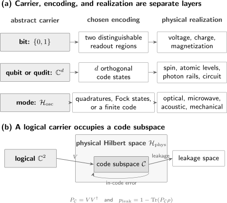
An information carrier is specified at more than one layer. The upper panel gives representative abstract carriers, encodings, and physical realizations; the arrows are examples rather than identities. The lower panel shows a logical carrier embedded isometrically in a physical Hilbert space. Noise may act within the code subspace or drive the state into leakage space.

This layered description prevents two common category errors. First, a device with many energy levels is not literally a two-level system merely because two levels are selected for control. Second, an abstract two-dimensional code space is not automatically protected: protection depends on the noise, syndrome information, recovery operations, and measured logical performance.

Classical Bits

A symbol, a random variable, and a storage element

The abstract classical bit alphabet is

$$\mathcal X=\{0,1\}.$$

A deterministic bit is one selected symbol $x\in\mathcal X$. A random bit is instead a probability distribution

$$p(0)=p, \qquad p(1)=1-p.$$

Its Shannon entropy is

$$H(X) = -p\log_2p -(1-p)\log_2(1-p),$$

which ranges from $0$ bits for a known value to $1$ bit for a uniform random bit. The word bit thus appears in at least three related senses:

• a two-symbol alphabet;
• a unit of classical information measured with a base-$2$ logarithm;
• a physical storage element designed to realize two reliably distinguishable states.

These senses should not be silently interchanged. A biased random bit has a two-element alphabet but entropy below one bit. A memory cell may have more microscopic states than its two logical macrostates. Error-correcting storage may use many physical cells for one protected logical bit.

Physical distinguishability

An ideal classical memory uses states that can be read without ambiguity at the chosen level of description. Real devices use separated regions of a noisy state space: two voltage ranges, two magnetization directions, two charge configurations, or two optical intensities. A decoder maps the analog readout to $0$ or $1$.

The physical variable need not itself be discrete. What makes the encoding a bit is the declared pair of codewords and the readout rule. Reliability is set by overlap of readout distributions, thermal activation, drift, retention time, and correction overhead, not by the symbol names.

For $n$ classical bits, the register alphabet has size

$$\lvert\mathcal X_n\rvert=2^n.$$

At any instant an ideal deterministic register occupies one of those $2^n$ configurations. A probability distribution over configurations represents uncertainty or deliberate randomization. This contrasts with a pure $n$-qubit state, which may contain coherent amplitudes over the same labels. Coherent amplitudes do not make all labels simultaneously readable.

Qubits

The abstract two-dimensional carrier

A qubit is a quantum system whose information-bearing Hilbert space is isomorphic to

$$\mathcal H_2\cong\mathbb C^2.$$

After choosing an orthonormal computational basis $\{|0\rangle,|1\rangle\}$, a pure state can be written

$$|\psi\rangle = \alpha|0\rangle+\beta|1\rangle, \qquad |\alpha|^2+|\beta|^2=1.$$

Vectors that differ by an overall phase represent the same pure state:

$$|\psi\rangle \sim e^{i\chi}|\psi\rangle.$$

The computational basis is part of an encoding convention, not a preferred basis imposed by the definition of a qubit. Another orthonormal pair can serve as the logical basis. Quantum States owns the general ray and density-operator formalism; the later Bloch-sphere page will own the geometric representation.

The coefficients $\alpha$ and $\beta$ are probability amplitudes. A computational-basis measurement has probabilities

$$p(0)=|\alpha|^2, \qquad p(1)=|\beta|^2,$$

but the state contains more operational structure than this one probability distribution. Relative phase affects measurements in other bases and interference under later transformations.

A qubit is not two classical bits

The pair of complex amplitudes does not permit arbitrary classical data to be extracted from one qubit. A measurement returns an outcome from its declared outcome set, and incompatible measurements generally disturb later statistics. Unknown nonorthogonal states cannot be perfectly distinguished in one shot, and No-Cloning and No-Signaling forbids a universal device that copies an arbitrary unknown qubit.

A qubit can nevertheless do things a classical bit cannot. It can preserve relative phase, become entangled with another system, and be transformed in bases that have no joint classical refinement. The operational consequences depend on a protocol; “being in superposition” alone is not an advantage claim.

Registers and tensor products

An $n$-qubit register has Hilbert space

$$\mathcal H_{2}^{\otimes n} \cong \mathbb C^{2^n}.$$

The computational basis is indexed by bit strings:

$$|x\rangle = |x_1\rangle\otimes\cdots\otimes|x_n\rangle, \qquad x\in\{0,1\}^n.$$

A general pure state is

$$|\Psi\rangle = \sum_{x\in\{0,1\}^n} c_x|x\rangle, \qquad \sum_x|c_x|^2=1.$$

The exponential dimension is a statement about state-space geometry and simulation cost. It is not permission to read out $2^n$ arbitrary classical numbers from one preparation. Algorithms gain value only when controlled dynamics and measurements make a task-relevant property accessible. Tensor Products gives the canonical composition rules.

Qudits

A qudit is a $d$-dimensional quantum carrier,

$$\mathcal H_d\cong\mathbb C^d, \qquad d\geq2,$$

with a chosen computational basis

$$\{|0\rangle,|1\rangle,\ldots,|d-1\rangle\}.$$

A pure state has the form

$$|\psi\rangle = \sum_{j=0}^{d-1}c_j|j\rangle, \qquad \sum_{j=0}^{d-1}|c_j|^2=1.$$

A qubit is the case $d=2$; a qutrit is the case $d=3$. Qudits arise naturally from atomic angular-momentum manifolds, multilevel ions, molecular rotational states, photon paths or time bins, orbital angular momentum, and controlled levels of nonlinear circuits.

Dimension accounting

Dimensions multiply under composition:

$$\dim(\mathcal H_A\otimes\mathcal H_B) = d_A d_B.$$

It is often useful to express a finite dimension in qubit-equivalent log-dimension

$$n_{\mathrm{dim}}=\log_2 d.$$

This is bookkeeping, not automatically a communication capacity or an experimentally accessible number of bits. A single $d$-level system supports at most $d$ mutually orthogonal codewords. What can actually be communicated depends on the state ensemble, prior probabilities, channel, receiver, error criterion, and resource accounting.

There is an exact Hilbert-space equivalence between one $d$-level carrier and an $n$-qubit register only when

$$d=2^n.$$

For example,

$$\mathbb C^4\cong\mathbb C^2\otimes\mathbb C^2,$$

but a qutrit is not exactly one and a half qubits. A qutrit can be embedded into two qubits with one unused basis state, or several qutrits can be encoded into qubit registers at an asymptotic rate approaching $\log_2 3$ qubits per qutrit. Those encodings have constraints and overhead.

Why use qudits?

Higher-dimensional carriers can match a system’s natural level structure, reduce the number of physical subsystems, or make some gates and codes more economical. They can also make calibration, selective control, readout, and leakage more difficult. The relevant comparison is therefore end to end:

$$\begin{gathered} \text{useful logical performance} \\ \text{at fixed accuracy, time, and resources}. \end{gathered}$$

not simply the Hilbert-space dimension per component.

Continuous-Variable Modes

One mode, infinitely many number states

A bosonic mode is commonly described by annihilation and creation operators $a$ and $a^\dagger$ satisfying

$$[a,a^\dagger]=1.$$

Its Fock basis is

$$\{|0\rangle,|1\rangle,|2\rangle,\ldots\},$$

with number operator

$$\hat n=a^\dagger a, \qquad \hat n|n\rangle=n|n\rangle.$$

The ideal mode Hilbert space is infinite dimensional. The label continuous variable refers to canonical observables such as dimensionless quadratures

$$\begin{aligned} \hat q &= \frac{a+a^\dagger}{\sqrt2}, \\ \hat p &= \frac{a-a^\dagger}{i\sqrt2}, \\ [\hat q,\hat p] &=i. \end{aligned}$$

whose measurement outcomes are continuous. The same mode has a discrete number basis. “Continuous-variable system” and “continuous energy spectrum” are therefore not synonyms.

Optical, microwave, acoustic, and mechanical normal modes are examples. A mode is not the same object as a particle: the state $|n\rangle$ describes $n$ excitations of one mode, while a single excitation can be distributed across several modes. Mode Occupations develops this distinction, and Continuous-Variable Systems owns the broader canonical formalism.

Infinite dimension does not mean infinite usable information

The ideal mode contains arbitrarily high number states, but physical tasks impose constraints. A common energy constraint is finite mean excitation number,

$$\langle\hat n\rangle_\rho = \operatorname{Tr}(\rho\hat n) \leq \bar n.$$

Bandwidth, preparation time, detector range, nonlinearity, loss, and available squeezing impose further limits. Without an energy or amplitude constraint, statements about capacities and approximation errors can become physically misleading.

Numerical calculations often truncate the Fock basis at $N$:

$$\mathcal H_{\leq N} = \operatorname{span} \{|0\rangle,\ldots,|N\rangle\}.$$

This is an approximation, not a change in the physical definition of the mode. A trustworthy calculation reports $N$ and verifies convergence of observables or bounds the omitted probability

$$\epsilon_N = \operatorname{Tr} \left[ (I-P_{\leq N})\rho \right].$$

Modes can host discrete encodings

An oscillator need not carry continuous-variable information directly. One may choose a two-dimensional subspace and encode a qubit. Examples include:

• Fock encodings using selected number states;
• cat codes using superpositions of coherent states;
• binomial codes using finite superpositions of number states;
• Gottesman–Kitaev–Preskill encodings using grid-like states in phase space.

The physical Hilbert space remains infinite dimensional while the logical carrier is finite dimensional. The distinction between carrier and encoding is doing real work here.

Physical, Encoded, and Logical Qubits

Physical qubits are controlled subsystems

A physical qubit is a physical degree of freedom used as the elementary qubit in an architecture. It may be:

• two spin projections in a fixed orbital manifold;
• two hyperfine or electronic states of an atom or ion;
• the lowest two levels of an anharmonic superconducting circuit;
• two photon polarizations, paths, or time bins;
• a pair of charge configurations;
• a two-state subspace of a larger oscillator or collective mode.

The full device Hilbert space is usually larger than $\mathbb C^2$. Selecting states $|0\rangle_{\mathrm p}$ and $|1\rangle_{\mathrm p}$ defines a physical-qubit subspace

$$\mathcal C_{\mathrm p} = \operatorname{span} \{|0\rangle_{\mathrm p},|1\rangle_{\mathrm p}\}.$$

Control pulses, noise, and measurement may couple this subspace to unused levels. Treating the device as an ideal qubit is justified only on timescales and at accuracies where those couplings are negligible or explicitly modeled.

Leakage is different from an in-code error

For a state $\rho$ in the full physical Hilbert space, the probability outside the declared code subspace is

$$p_{\mathrm{leak}} = 1-\operatorname{Tr} \left(P_{\mathcal C}\rho\right).$$

An error that maps $|0\rangle$ to $|1\rangle$ remains inside the qubit subspace. Leakage instead transfers population to states outside it, such as $|2\rangle$ of a weakly anharmonic circuit, vacuum in a single-photon encoding, or an unwanted atomic level. These errors require different models and recovery mechanisms. Erasure and Loss Channels gives the channel-level treatment when loss is flagged or represented by an orthogonal erasure state.

Conditioning on remaining in the code gives

$$\rho_{\mathcal C} = \frac{ P_{\mathcal C}\rho P_{\mathcal C} }{ \operatorname{Tr}(P_{\mathcal C}\rho) },$$

provided the denominator is nonzero. Reporting only this conditional state can hide leakage. Device characterization should report both survival probability and conditional quality.

Encoded qubits

An encoded qubit is any isometric embedding

$$V:\mathbb C^2\longrightarrow\mathcal H_{\mathrm{phys}}.$$

Its logical basis states are

$$|0_L\rangle=V|0\rangle, \qquad |1_L\rangle=V|1\rangle.$$

A logical operator $\bar U$ acts on the code as the desired abstract operation:

$$\bar U V=VU.$$

This definition covers both protected and unprotected embeddings. For example, the dual-rail photonic encoding uses two modes:

$$|0_L\rangle=|1,0\rangle, \qquad |1_L\rangle=|0,1\rangle.$$

The one-photon sector is the code space. Losing the photon produces $|0,0\rangle$, which is orthogonal to the code and can be interpreted as erasure when detected.

Logical qubits and protection

Usage varies across the literature: some authors call every code-space degree of freedom a logical qubit, while others reserve logical qubit for an actively error-corrected object. Here the term means an encoded qubit addressed through logical operations, with the degree of protection stated explicitly. “Logical” alone does not prove fault tolerance.

For oscillator encodings, Bosonic and Encoded Computation Models takes the declared carrier-to-code map as input and derives the operation induced by a complete physical program, including leakage, rejection, recovery, frames, and resources. This page retains the carrier, state, device, code-subspace, and logical-encoding distinctions themselves.

For an $n$-physical-qubit code encoding $k$ qubits, the code subspace has dimension

$$\dim\mathcal C=2^k$$

inside

$$\dim\mathcal H_{\mathrm{phys}}=2^n.$$

The redundancy allows selected errors to move the state into distinguishable syndrome sectors without revealing the encoded amplitudes. A code is useful only relative to an error model and available recovery operations.

The three-qubit repetition encoding illustrates both the possibility and the limitation:

$$\begin{aligned} |0_L\rangle&=|000\rangle, \\ |1_L\rangle&=|111\rangle, \\ \alpha|0\rangle+\beta|1\rangle &\longmapsto \alpha|000\rangle+\beta|111\rangle. \end{aligned}$$

This code can diagnose and correct one bit flip when suitable syndrome measurements and recovery are available. It does not correct an arbitrary one-qubit error and does not protect against a phase flip. The map also does not clone the unknown state: the encoded superposition is generally entangled, and none of the three individual qubits has state $\alpha|0\rangle+\beta|1\rangle$.

Full quantum error correction requires more than redundancy. A protected logical architecture needs:

• a declared code and correctable error set;
• syndrome extraction that does not reveal logical information;
• a decoder and recovery or tracked correction;
• logical state preparation, gates, and measurement;
• treatment of leakage, loss, correlated errors, and faulty correction circuitry;
• evidence that logical error decreases as the code or resources are increased in the claimed regime.

Why Quantum Error Correction Is Possible gives the exact correctability criterion and explains why syndrome information need not reveal the logical state. Three-Qubit Codes owns the concrete bit- and phase-flip repetition encodings, syndrome sectors, ideal recoveries, and restricted-distance limits; this page retains the carrier, code-subspace, encoding-isometry, and no-cloning distinctions.

Representative Encodings

Abstract carrier	Encoding or code space	Representative physical realization	Important out-of-code process
Classical bit	Two disjoint readout regions	Voltage, magnetization, charge, optical intensity	Ambiguous threshold crossing or state loss
Qubit	Two selected energy or spin states	Atom, ion, spin, superconducting circuit	Excitation to unused levels
Qubit	One photon in two modes	Polarization, path, time-bin, or frequency-bin rails	Vacuum after photon loss
Qudit	$d$ selected orthogonal states	Atomic manifold, multilevel ion, photonic paths	Transfer outside selected manifold
CV mode	Full oscillator state space under an energy constraint	Optical, microwave, acoustic, or mechanical mode	Loss, saturation, bandwidth truncation
Bosonic logical qubit	Two-dimensional code in one or more modes	Cat, binomial, or GKP code	Uncorrectable shift, loss, or escape from code manifold

This table is a taxonomy, not a ranking. “More levels” does not automatically mean “more useful information,” and “logical” does not automatically mean “better.” Performance must be compared for a task under matched constraints.

Hybrid Encodings and Interfaces

Hybrid can describe several distinct architectures.

Discrete information in a continuous-variable system

A qubit encoded in an oscillator is discrete logical information hosted by continuous-variable hardware. The logical dimension is two even though the physical mode is infinite dimensional. Bosonic codes exploit the mode’s larger state space to make common errors detectable or correctable. Bosonic Qubits develops the resulting module architecture, nonlinear-control requirements, syndrome paths, benchmarks, and physical-resource ledger.

Different carrier types in one processor

An ion’s internal levels may store qubits while collective vibrational modes mediate gates. A superconducting circuit may control a microwave cavity that stores a bosonic code. A photon may transport a qubit between stationary matter qubits. In each case, the subsystems have different noise, lifetime, control, and measurement models.

Transduction between encodings

A network may need to map

$$\begin{gathered} \text{microwave excitation} \\ \longleftrightarrow \\ \text{optical excitation} \end{gathered}$$

or

$$\begin{gathered} \text{stationary matter qubit} \\ \longleftrightarrow \\ \text{flying photonic qubit}. \end{gathered}$$

An ideal transducer preserves the logical state while changing the physical carrier. Real interfaces add loss, thermal noise, mode mismatch, limited bandwidth, and phase instability. Interconnects and Transduction develops the complete physical-channel and service contract. The correct metric is a channel-level figure of merit for the intended ensemble and task, not conversion efficiency alone.

Classical side information is not a hybrid quantum encoding

Quantum protocols routinely use classical control records, calibration parameters, detector timestamps, and syndrome bits. Their presence does not by itself make the quantum carrier hybrid. A hybrid encoding uses more than one physical or mathematical carrier type for the quantum information itself, or coherently maps between them.

How to Choose a Carrier

Carrier selection is an architecture decision, not a contest over which system is “most quantum.” Relevant questions include:

1. State space: Is the natural object a qubit, qudit, mode, or encoded subsystem?
2. Initialization: Can the required code states be prepared with known error?
3. Control: Which transformations are native, and which require long compiled sequences?
4. Readout: Is measurement destructive, number resolving, basis selective, or naturally heralded?
5. Noise: Are dephasing, relaxation, loss, leakage, thermal occupation, or correlated errors dominant?
6. Connectivity: Which subsystems interact directly, and at what crosstalk cost?
7. Timescale: How do gate, measurement, reset, communication, and coherence times compare?
8. Scalability: What wiring, lasers, cryogenics, fabrication, calibration, and classical processing are required?
9. Encoding overhead: How many physical resources and correction cycles are needed per useful logical carrier?
10. Verification: Which physical and logical quantities can be estimated independently?

A two-level approximation may simplify control but waste useful levels. A qudit may compactly represent a local degree of freedom but demand more precise addressing. A bosonic code may reduce component count while requiring high-quality oscillators and nonlinear ancillas. A photonic qubit may travel well but be difficult to store or interact deterministically. There is no platform-independent answer.

Common Mistakes

“A qubit is both 0 and 1”

A qubit is a state in a two-dimensional Hilbert space. A superposition has amplitudes relative to a basis; it is not a classical register simultaneously holding two readable values.

“An $n$-qubit state stores $2^n$ accessible numbers”

A state description may require exponentially many amplitudes, but one measurement returns limited classical data. Learning an arbitrary unknown state requires many preparations and measurement settings. Computational value comes from task structure.

“A device with two labeled levels is exactly a qubit”

Most physical devices have additional states. The qubit model is an effective description whose leakage, initialization, controls, and readout errors must be checked.

“An encoded qubit is automatically error corrected”

Encoding creates a code subspace. Protection additionally requires that relevant errors be detectable or correctable and that recovery operations improve the logical performance under realistic faults.

“A logical error rate can be compared directly with any physical error rate”

The quantities must refer to matched operations, durations, noise conditions, and success criteria. A logical memory cycle, logical gate, and physical gate are different experiments.

“A mode carries infinite usable information”

The ideal Hilbert space is infinite dimensional, but energy, bandwidth, noise, preparation, and measurement constraints limit every physical task.

“A qutrit is exactly 1.585 qubits”

$\log_2 3$ is useful dimension bookkeeping and an asymptotic coding rate. It is not an exact decomposition of one qutrit into a fractional number of qubit subsystems.

Exercises

1. Dimension bookkeeping

A register contains two qubits, one qutrit, and one oscillator truncated to number states $|0\rangle$ through $|5\rangle$. What is the dimension of the modeled Hilbert space? How many qubits are required for a direct binary embedding with no compression assumptions?

Solution

The subsystem dimensions are $2$, $2$, $3$, and $6$. Tensor-product dimensions multiply:

$$D=2\cdot2\cdot3\cdot6=72.$$

An $n$-qubit register has dimension $2^n$. Since

$$2^6=64<72\leq128=2^7,$$

seven qubits are required for a direct embedding. The embedding has $128-72=56$ unused basis states. This count concerns the chosen truncated model; the untruncated oscillator is infinite dimensional.

2. When is a qudit a qubit register?

For which values of $d$ can a single qudit be identified exactly with an $n$-qubit tensor-product register without unused states? Explain why $d=6$ does not qualify, even though $\log_2 6$ is well defined.

Solution

Exact equality of dimensions requires

$$d=2^n$$

for an integer $n\geq0$. In that case an isomorphism can map the qudit basis to $n$-bit strings.

For $d=6$,

$$\log_2 6\approx2.585,$$

which is not an integer. Three qubits can host a six-dimensional code subspace, but two of their eight computational-basis states remain unused. The logarithm measures dimension on a base-$2$ scale; it does not construct fractional tensor factors.

3. Leakage and conditional quality

A three-level device uses $|0\rangle$ and $|1\rangle$ as its physical-qubit subspace. After a gate,

$$\rho = 0.45|0\rangle\langle0| + 0.45|1\rangle\langle1| + 0.10|2\rangle\langle2|.$$

Find the leakage probability and the state conditioned on remaining in the qubit subspace. Why is the conditional state alone an incomplete report?

Solution

With

$$P_{\mathcal C} = |0\rangle\langle0| + |1\rangle\langle1|,$$

the survival probability is

$$\operatorname{Tr}(P_{\mathcal C}\rho)=0.90,$$

so

$$p_{\mathrm{leak}}=1-0.90=0.10.$$

Conditioning and renormalizing gives

$$\rho_{\mathcal C} = \frac1{0.90} \left( \begin{aligned} &0.45|0\rangle\langle0| \\ &+0.45|1\rangle\langle1| \end{aligned} \right).$$

Equivalently,

$$\rho_{\mathcal C} = \frac12 \left( |0\rangle\langle0| + |1\rangle\langle1| \right).$$

This normalized state discards the ten-percent failure probability. A complete report gives both survival and conditional state quality.

4. Loss in a dual-rail qubit

A dual-rail state is

$$|\psi_L\rangle = \alpha|1,0\rangle+\beta|0,1\rangle.$$

Both rails have the same single-photon transmissivity $\eta$. Show that the output is a mixture of the unchanged logical state and vacuum. What happens when one conditions on detecting that a photon survived?

Solution

Equal loss on the two modes does not reveal which rail carried the photon. The one-photon component survives with probability $\eta$, while loss produces the vacuum with probability $1-\eta$:

$$\rho_{\mathrm{out}} = \eta|\psi_L\rangle\langle\psi_L| + (1-\eta)|0,0\rangle\langle0,0|.$$

The vacuum is orthogonal to the code space

$$\operatorname{span}\{|1,0\rangle,|0,1\rangle\}.$$

Conditioned on a verified one-photon event, the normalized logical state remains $|\psi_L\rangle$. Without conditioning, the channel has an erasure probability $1-\eta$. Unequal rail transmissivities would also distort the relative amplitudes in the surviving component.

5. What the repetition code protects

Encode

$$|\psi\rangle=\alpha|0\rangle+\beta|1\rangle$$

as

$$|\psi_L\rangle = \alpha|000\rangle+\beta|111\rangle.$$

Apply a bit flip $X_2$ to the middle qubit and compute the eigenvalues of the parity checks $Z_1Z_2$ and $Z_2Z_3$. Then apply a phase flip $Z_1$ to the original codeword. What does this show?

Solution

The middle-qubit flip gives

$$X_2|\psi_L\rangle = \alpha|010\rangle+\beta|101\rangle.$$

Both parity checks change sign:

$$Z_1Z_2=-1, \qquad Z_2Z_3=-1$$

on this error sector. The syndrome identifies the middle qubit without measuring $\alpha$ or $\beta$, so applying $X_2$ recovers the codeword.

A phase flip gives

$$Z_1|\psi_L\rangle = \alpha|000\rangle-\beta|111\rangle.$$

This state still has eigenvalue $+1$ for both $Z$-parity checks. The error acts as a logical phase flip and is not corrected by the repetition code. The code protects against one selected error type, not arbitrary noise.

6. Finite energy and Fock truncation

Let a mode state have finite mean occupation

$$\langle\hat n\rangle=\bar n.$$

Show that the probability of finding $n\geq N+1$ obeys

$$\Pr(n\geq N+1) \leq \frac{\bar n}{N+1}.$$

What does the bound say about numerical truncation?

Solution

Let $p_n=\langle n|\rho|n\rangle$. For all terms with $n\geq N+1$,

$$n\geq N+1.$$

Therefore

$$\begin{aligned} \bar n &= \sum_{n=0}^{\infty}np_n \\ &\geq \sum_{n=N+1}^{\infty}np_n \\ &\geq (N+1) \sum_{n=N+1}^{\infty}p_n. \end{aligned}$$

Rearranging gives

$$\epsilon_N = \sum_{n=N+1}^{\infty}p_n \leq \frac{\bar n}{N+1}.$$

Finite mean energy guarantees that the omitted probability can be made small by increasing $N$, but this general bound can be loose. A numerical study should inspect convergence or use tighter information about the state rather than assume a small cutoff is adequate.

Where to Go Next

• Information-Theoretic Foundations decides whether a question is about a carrier, encoded state, process, measurement, information measure, or resource before routing it to the corresponding owner.
• Classical Information Review fixes the alphabet, source, channel, code, decoder, and cost baseline before a carrier-level quantum comparison; this page owns the carrier and encoding distinctions.
• Quantum Information and Computation maps carriers into the larger computation, communication, sensing, simulation, and fault-tolerance stack.
• Bloch Sphere for Quantum Information is the next operational step for one-qubit states, measurements, gates, and channels.
• Single-Qubit Gates develops the ideal transformations available on a chosen qubit basis and connects them to physical controls.
• Circuit Model explains how carriers become ordered registers connected by gates, measurements, and classical control.
• Reversible Computation explains when a logical map is bijective and how classical functions become reversible embeddings with explicit workspace, garbage, and cleanup.
• What Is Quantum Information? introduces the operational task language in which a carrier becomes useful.
• Quantum Information Roadmap gives the staged learning path through the volume.
• Math Needed for Quantum Information reviews complex vector spaces, tensor products, probability, and entropy.
• Quantum States owns the general state and ray formalism.
• Density Operators treats mixed states and reduced descriptions.
• Two-Level Systems develops the canonical dynamics of a physical two-level model.
• Photon Number States develops Fock states and optical number statistics.
• Trapped-Ion Control illustrates internal-state qubits coupled through motional modes.
• Quantum Channels and Noise supplies the canonical process language for loss, decoherence, and leakage-aware models.

References

• C. E. Shannon, “A mathematical theory of communication,” Bell System Technical Journal 27, 379–423 and 623–656, 1948, doi:10.1002/j.1538-7305.1948.tb01338.x.
• M. A. Nielsen and I. L. Chuang, Quantum Computation and Quantum Information, 10th anniversary ed., Cambridge University Press, 2010, doi:10.1017/CBO9780511976667.
• J. Watrous, The Theory of Quantum Information, Cambridge University Press, 2018, doi:10.1017/9781316848142.
• M. M. Wilde, Quantum Information Theory, 2nd ed., Cambridge University Press, 2017, doi:10.1017/9781316809976.
• J. Preskill, Lecture Notes for Physics 219/Computer Science 219: Quantum Computation, California Institute of Technology, course materials.
• B. Schumacher, “Quantum coding,” Physical Review A 51, 2738–2747, 1995, doi:10.1103/PhysRevA.51.2738.
• D. P. DiVincenzo, “The physical implementation of quantum computation,” Fortschritte der Physik 48, 771–783, 2000, doi:10.1002/1521-3978(200009)48:9/11%3C771::AID-PROP771%3E3.0.CO;2-E.
• E. Knill and R. Laflamme, “Theory of quantum error-correcting codes,” Physical Review A 55, 900–911, 1997, doi:10.1103/PhysRevA.55.900.
• B. M. Terhal, “Quantum error correction for quantum memories,” Reviews of Modern Physics 87, 307–346, 2015, doi:10.1103/RevModPhys.87.307.
• S. L. Braunstein and P. van Loock, “Quantum information with continuous variables,” Reviews of Modern Physics 77, 513–577, 2005, doi:10.1103/RevModPhys.77.513.
• C. Weedbrook, S. Pirandola, R. García-Patrón, N. J. Cerf, T. C. Ralph, J. H. Shapiro, and S. Lloyd, “Gaussian quantum information,” Reviews of Modern Physics 84, 621–669, 2012, doi:10.1103/RevModPhys.84.621.
• D. Gottesman, A. Kitaev, and J. Preskill, “Encoding a qubit in an oscillator,” Physical Review A 64, 012310, 2001, doi:10.1103/PhysRevA.64.012310.
• W. Cai, Y. Ma, W. Wang, C.-L. Zou, and L. Sun, “Bosonic quantum error correction codes in superconducting quantum circuits,” Fundamental Research 1, 50–67, 2021, doi:10.1016/j.fmre.2020.12.006.
• G. Wendin, “Quantum information processing with superconducting circuits: a review,” Reports on Progress in Physics 80, 106001, 2017, doi:10.1088/1361-6633/aa7e1a.
• D. Leibfried, R. Blatt, C. Monroe, and D. Wineland, “Quantum dynamics of single trapped ions,” Reviews of Modern Physics 75, 281–324, 2003, doi:10.1103/RevModPhys.75.281.

Summary

Bits, qubits, qudits, and modes are abstract carrier types, not hardware brands. A bit uses two distinguishable classical symbols; a qubit uses a two-dimensional Hilbert space; a qudit uses $d$ dimensions; and a continuous-variable mode uses an infinite-dimensional oscillator space subject to physical constraints. Tensor-product dimensions multiply, while $\log_2 d$ provides dimension bookkeeping without by itself specifying capacity or accessible information.

An encoding is an isometry into a physical Hilbert space. Its image defines a code subspace, and population outside that subspace is leakage. Physical qubits are elementary controlled systems; encoded qubits are chosen two-dimensional subspaces; logical qubits are manipulated at the code level and must have their actual protection stated. Hybrid architectures combine or transduce between carrier types. Trustworthy comparisons therefore name the encoding, physical realization, noise model, resource constraints, and logical task.