Density Operators for Quantum Information

Short Definition

A density operator is the state object used when a quantum-information task involves preparation uncertainty, discarded subsystems, entanglement, noise, measurement branches, or communication ensembles. On a finite-dimensional Hilbert space $\mathcal H$, it satisfies

$$\rho^\dagger=\rho, \qquad \rho\geq0, \qquad \operatorname{Tr}\rho=1.$$

It predicts every measurement probability through

$$\begin{aligned} p(y) &= \operatorname{Tr}(M_y\rho), \\ M_y&\geq0, \qquad \sum_yM_y=I. \end{aligned}$$

and every observable expectation through

$$\langle A\rangle = \operatorname{Tr}(\rho A).$$

Density Operators is the canonical home for the general definition and postulates. This page owns the operational QI workflow: how $\rho$ arises from sources and subsystems, how channels and instruments transform it, how fidelity and trace distance compare it, how purification represents it, and how a calculation or experiment checks that a proposed matrix is physically meaningful.

Why QI Uses Density Operators by Default

A state vector is sufficient for a closed system known to be pure. Most information-processing descriptions are not in that situation. A density operator is needed when:

• a source prepares several signals with declared probabilities;
• only one part of an entangled register is available;
• an environment, ancilla, measurement record, or classical label is discarded;
• a noisy channel maps pure inputs to mixed outputs;
• a protocol conditions on a measurement outcome;
• a tomography procedure estimates a state from finite data;
• a receiver must distinguish an ensemble of nonorthogonal signals;
• an algorithm’s output is evaluated only on a subsystem.

These cases have different physical origins, but they share the same local probability rule. The density operator is not a claim that every mixed state is “really” an unknown pure state. It is the complete state description for the observables assigned to the system under consideration.

Three Layers of Meaning

The operator

At the mathematical layer, $\rho$ is a positive trace-one operator. Positivity means

$$\langle\psi|\rho|\psi\rangle\geq0$$

for every $|\psi\rangle$. Equivalently in finite dimension, all eigenvalues are nonnegative. The trace-one condition normalizes total probability.

The preparation

A laboratory preparation procedure may be described by an ensemble

$$\mathcal E = \{p_x,\rho_x\}_x.$$

If the label $x$ is not retained, the emitted system is described by the average state

$$\bar\rho = \sum_xp_x\rho_x.$$

Different ensembles can have the same average. No measurement on the emitted system alone can determine which ensemble decomposition was used when the density operators agree.

The information available to an observer

If the classical label is retained in a register $X$, the joint classical–quantum state is

$$\rho_{XB} = \sum_x p_x |x\rangle\langle x|_X \otimes \rho_B^x.$$

Discarding $X$ gives

$$\rho_B = \operatorname{Tr}_X\rho_{XB} = \sum_xp_x\rho_B^x.$$

The states $\rho_{XB}$ and $\rho_B$ do not contain the same information. The first preserves which signal was selected; the second describes a receiver who has only the quantum system. This distinction underlies coding, state discrimination, cryptography, and the Holevo information.

Spectra, Rank, and Purity

Every finite-dimensional density operator has a spectral decomposition

$$\begin{aligned} \rho &= \sum_{j=1}^{r} \lambda_j |j\rangle\langle j|, \\ \lambda_j&>0, \qquad \sum_j\lambda_j=1. \end{aligned}$$

where $r=\operatorname{rank}\rho$. This decomposition is orthogonal and is fixed by $\rho$ up to basis choices inside degenerate eigenspaces. It should not be confused with a general preparation ensemble, whose states may be nonorthogonal and whose decomposition is highly nonunique.

A state is pure exactly when

$$\rho^2=\rho,$$

or equivalently

$$\operatorname{Tr}(\rho^2)=1.$$

The purity

$$\gamma(\rho) = \operatorname{Tr}(\rho^2) = \sum_j\lambda_j^2$$

obeys

$$\frac1d \leq \gamma(\rho) \leq 1$$

in dimension $d$. The lower bound is attained by $I/d$.

Purity is a useful diagnostic, but it is not a distance to a target state and it does not identify the noise mechanism. Two states can have equal purity and be far apart. Purities from different Hilbert-space dimensions also have different lower bounds. Pure vs Mixed States owns the conceptual distinction between rays, coherent superpositions, and mixtures.

One-qubit representation

For one qubit,

$$\rho = \frac12 \left( I+\mathbf r\cdot\boldsymbol\sigma \right), \qquad \lVert\mathbf r\rVert\leq1,$$

and

$$\gamma(\rho) = \frac{ 1+\lVert\mathbf r\rVert^2 }{2}.$$

Bloch Sphere for Quantum Information is the canonical QI home for the one-qubit operational geometry, tomography axes, gate rotations, and affine channel maps. The Bloch representation does not generalize to a simple ball for higher-dimensional states.

Density Operators from Composite Systems

Reduced states

For a bipartite state $\rho_{AB}$, the state available to an observer with access only to $A$ is

$$\rho_A = \operatorname{Tr}_B\rho_{AB}.$$

It is characterized by the requirement

$$\operatorname{Tr} \left[ \rho_{AB} (M_A\otimes I_B) \right] = \operatorname{Tr} \left( \rho_A M_A \right)$$

for every local effect or observable $M_A$. Thus $\rho_A$ contains exactly the statistics of measurements on $A$ alone.

If

$$|\Phi^+\rangle_{AB} = \frac{ |00\rangle+|11\rangle }{\sqrt2},$$

then

$$\rho_A=\rho_B=\frac I2$$

even though $\rho_{AB}=|\Phi^+\rangle\langle\Phi^+|$ is pure. Local mixedness can arise from entanglement, not from classical uncertainty about a hidden local pure state. Partial Trace owns the basis-independent definition, index rules, and full calculations.

Discarding is a channel

The map

$$\operatorname{Tr}_B: \mathcal L(\mathcal H_A\otimes\mathcal H_B) \longrightarrow \mathcal L(\mathcal H_A)$$

is a quantum channel. Operationally, “ignore the ancilla,” “do not read the environment,” and “keep only the output register” are partial-trace instructions. They can turn a pure global state into a mixed local state while preserving all local probabilities.

This is why an algorithmic derivation must state which registers are retained. A final state vector for the full circuit is not yet the answer when the task asks for one output register.

Purification

Every density operator can be realized as the reduced state of a pure state on a larger system. From the spectral decomposition,

$$\rho_A = \sum_j\lambda_j|j\rangle\langle j|,$$

one purification is

$$|\Psi\rangle_{AR} = \sum_j \sqrt{\lambda_j} |j\rangle_A|j\rangle_R.$$

Tracing out the reference gives

$$\operatorname{Tr}_R \left( |\Psi\rangle\langle\Psi| \right) = \rho_A.$$

The reference dimension need be no larger than $\operatorname{rank}\rho_A$. Purifications are not unique: two purifications of the same state are related by an isometry on the purifying system, with a unitary sufficient when the reference spaces have equal dimension.

Purification is not an assertion that an accessible hidden ancilla physically exists in every experiment. It is a representation theorem and a powerful proof device. QI uses it to:

• analyze channels through unitary dilations;
• define entanglement fidelity and complementary channels;
• compare states through Uhlmann’s theorem;
• model an adversary holding a purification in security proofs;
• convert mixed-state questions into pure bipartite-state questions;
• construct matrix-product and tensor-network representations.

Purification owns the theorem, minimal purifying dimension, isometric freedom, and relation to Schmidt decomposition.

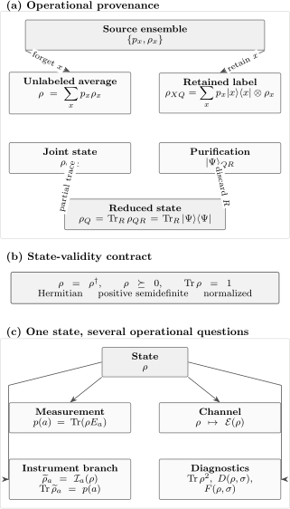
A density operator can arise by forgetting a source label or tracing out a subsystem. Once $\rho$ is specified, the same object feeds measurement probabilities, channel evolution, conditional instrument branches, and state diagnostics. Retaining a classical record or reference system gives a different joint state from averaging or discarding it.

Transformations in Protocols

Closed-system evolution

A unitary transformation acts by conjugation:

$$\rho \longmapsto U\rho U^\dagger.$$

It preserves the spectrum, rank, purity, and von Neumann entropy. A unitary cannot turn a mixed state into a pure state on the same isolated system.

Quantum channels

A quantum channel $\mathcal N$ is a completely positive trace-preserving linear map. In a Kraus representation,

$$\mathcal N(\rho) = \sum_aK_a\rho K_a^\dagger, \qquad \sum_aK_a^\dagger K_a=I.$$

The output is again a density operator. Channels describe intended gates with noise, communication links, discarded environments, reset, dephasing, loss models, and many protocol components. Quantum Channels and Noise owns the full Kraus, Choi, Stinespring, and complete-positivity machinery.

Quantum Channels for QI owns the finite-dimensional QI workflow for freezing conventions, converting representations, and composing maps; this page retains state, ensemble, marginal, purification, and subnormalized-branch bookkeeping.

Measurement branches are often subnormalized

A quantum instrument with outcome $m$ maps an input to

$$\widetilde\rho_m = \mathcal I_m(\rho).$$

The tilde marks a subnormalized positive operator:

$$p(m) = \operatorname{Tr}\widetilde\rho_m.$$

Conditioned on an outcome with nonzero probability, the normalized state is

$$\rho_m = \frac{ \widetilde\rho_m }{ p(m) }.$$

This bookkeeping matters in postselection, heralded entanglement, syndrome extraction, and quantum trajectories. Normalizing each branch too early erases its probability; failing to normalize before using $\rho_m$ as a state gives incorrect conditional expectations.

For one Kraus operator $M_m$ per branch,

$$\widetilde\rho_m = M_m\rho M_m^\dagger, \qquad \sum_mM_m^\dagger M_m=I.$$

The sum over outcomes,

$$\sum_m\widetilde\rho_m,$$

is the nonselective output state.

Comparing Quantum States

No single scalar answers every comparison question. The task determines the appropriate quantity.

Trace distance

The trace distance is

$$D(\rho,\sigma) = \frac12 \lVert\rho-\sigma\rVert_1.$$

It is a metric, ranges from $0$ to $1$, and controls optimal one-shot state discrimination. For equal priors,

$$P_{\mathrm{guess}} = \frac12 \left[ 1+D(\rho,\sigma) \right].$$

It is contractive under channels:

$$D \left( \mathcal N(\rho),\mathcal N(\sigma) \right) \leq D(\rho,\sigma).$$

Physical processing cannot make two states more distinguishable when the same channel is applied to both and no side information is added. Trace Distance is the formula card with assumptions and convention checks.

Several calculation shortcuts expose its meaning. For commuting states with eigenvalue distributions $p_i$ and $q_i$,

$$D(\rho,\sigma)=\frac12\sum_i|p_i-q_i|.$$

For two pure states,

$$D(|\psi\rangle,|\phi\rangle) =\sqrt{1-|\langle\psi|\phi\rangle|^2},$$

and for qubit Bloch vectors $\mathbf r$ and $\mathbf s$,

$$D(\rho,\sigma)=\frac12\lVert\mathbf r-\mathbf s\rVert_2.$$

The variational characterization

$$D(\rho,\sigma) =\max_{0\le M\le I} \operatorname{Tr}[M(\rho-\sigma)]$$

shows that trace distance is the largest difference in the probability of one measurement event. It also implies, for a bounded observable $A$,

$$|\operatorname{Tr}[A(\rho-\sigma)]| \le2\lVert A\rVert_\infty D(\rho,\sigma).$$

For prior probabilities $p$ and $1-p$, the optimal binary discrimination probability is

$$P_{\mathrm{guess}}^{\mathrm{opt}} =\frac12\left(1+ \lVert p\rho-(1-p)\sigma\rVert_1\right).$$

The equal-prior formula above is its $p=1/2$ specialization.

Fidelity

This site uses squared Uhlmann fidelity:

$$F(\rho,\sigma) = \left[ \operatorname{Tr} \sqrt{ \sqrt\rho\,\sigma\sqrt\rho } \right]^2.$$

It ranges from $0$ to $1$ and equals $1$ exactly when $\rho=\sigma$. If $\rho=|\psi\rangle\langle\psi|$ is pure,

$$F(\rho,\sigma) = \langle\psi|\sigma|\psi\rangle.$$

Fidelity is not a metric, and some references use the unsquared square-root quantity under the same name. The convention must accompany a reported value. Fidelity is the canonical formula card.

Useful special cases in the squared convention are

$$F(|\psi\rangle,|\phi\rangle) =|\langle\psi|\phi\rangle|^2,$$ $$F(\rho,\sigma) =\left(\sum_i\sqrt{p_iq_i}\right)^2$$

for commuting states, and

$$F(\rho,\sigma) =\frac12\left[ 1+\mathbf r\cdot\mathbf s +\sqrt{(1-\lVert\mathbf r\rVert^2) (1-\lVert\mathbf s\rVert^2)} \right]$$

for qubits. Fidelity is multiplicative on tensor products and monotone under a common channel:

$$F(\rho_1\otimes\rho_2,\sigma_1\otimes\sigma_2) =F(\rho_1,\sigma_1)F(\rho_2,\sigma_2),$$ $$F(\mathcal N(\rho),\mathcal N(\sigma)) \ge F(\rho,\sigma).$$

Uhlmann’s theorem gives the purification form

$$F(\rho,\sigma) =\max_{|\psi_\rho\rangle,|\psi_\sigma\rangle} |\langle\psi_\rho|\psi_\sigma\rangle|^2,$$

where the maximization is over purifications in a common larger space. Numerically, symmetrize estimated density matrices, reject substantial negative eigenvalues rather than silently clipping them, and use stable positive square-root routines.

For the squared convention, the Fuchs–van de Graaf inequalities are

$$\begin{aligned} 1-\sqrt{F(\rho,\sigma)} &\leq D(\rho,\sigma), \\ D(\rho,\sigma) &\leq \sqrt{1-F(\rho,\sigma)}. \end{aligned}$$

They translate bounds between two different notions of closeness; they do not make fidelity and trace distance interchangeable.

Purity, entropy, and target overlap answer different questions

Purity asks how concentrated the spectrum is. Fidelity asks closeness to a specified target. Trace distance asks distinguishability. Von Neumann entropy,

$$S(\rho) = -\operatorname{Tr} \left( \rho\log_2\rho \right),$$

quantifies spectral uncertainty and has several information-theoretic roles. A high-purity state can have zero fidelity with the desired pure target. A low trace distance to one target says nothing about closeness to another. The later quantum-entropy page owns entropy and its operational uses.

A Source Ensemble Example

Suppose a source emits $|0\rangle$ with probability $p$ and $|+\rangle$ with probability $1-p$, while withholding the label. The receiver’s state is

$$\begin{aligned} \bar\rho &= p|0\rangle\langle0| + (1-p)|+\rangle\langle+| \\ &= \frac12 \begin{pmatrix} 1+p&1-p \\ 1-p&1-p \end{pmatrix}. \end{aligned}$$

Its Bloch vector is

$$\mathbf r=(1-p,0,p),$$

and its purity is

$$\operatorname{Tr}(\bar\rho^2) = 1-p+p^2.$$

At $p=1/2$,

$$\bar\rho = \begin{pmatrix} 3/4&1/4 \\ 1/4&1/4 \end{pmatrix}, \qquad \operatorname{Tr}(\bar\rho^2)=\frac34.$$

The average is mixed because the two possible signals are distinct. It still has coherence in the computational basis because one ensemble member is $|+\rangle$. A mixed state need not be diagonal in the basis chosen for display.

If the source keeps the label $X$, the correct state is instead

$$\begin{aligned} \rho_{XB} &= p|0\rangle\langle0|_X \otimes |0\rangle\langle0|_B \\ &\quad+ (1-p)|1\rangle\langle1|_X \otimes |+\rangle\langle+|_B. \end{aligned}$$

This joint state permits correlations between the label and a later measurement outcome. Averaging to $\bar\rho_B$ intentionally discards those correlations.

Where Density Operators Enter QI

Algorithms and circuits

Density operators describe noisy initial states, reset errors, mixed ancillas, mid-circuit measurement branches, reduced output registers, and randomized circuit ensembles. An ideal pure-state derivation may use vectors internally, but a hardware-level prediction generally needs channels and density operators.

Communication and cryptography

A sender chooses an ensemble $\{p_x,\rho_x\}$; a receiver sees the average state unless side information reveals $x$. Distinguishability, accessible information, Holevo quantities, and security proofs are all density-operator statements. In adversarial analyses, a purifying reference often represents information held outside the honest subsystem.

Noise and error correction

Noise acts as a channel on $\rho$. Syndrome outcomes are instrument branches. Logical states are density operators supported on a code subspace, and uncorrectable faults can mix or leak them. Comparing the recovered state with the target requires a declared state or channel metric.

Tomography and benchmarking

Tomography estimates a positive trace-one matrix from frequencies. Benchmarking may compare estimated states, average outputs, or channels; these are not the same objects. State fidelity cannot by itself certify a gate on arbitrary inputs.

Simulation

Numerical open-system solvers propagate density matrices. Tensor-network and Monte Carlo methods may represent them directly, purify them, or sample trajectories whose average reproduces them. Each representation has different cost, bias, and convergence checks.

Numerical and Experimental Validity Checks

For a finite matrix proposed as a density operator, check:

1. Dimensions and basis order: identify every tensor factor and index convention.
2. Hermiticity: verify $\rho^\dagger=\rho$ within a stated tolerance.
3. Trace: verify $\operatorname{Tr}\rho=1$ for a normalized state.
4. Positivity: inspect the smallest eigenvalue or use a positive parameterization.
5. Purity and rank: report them when they matter, without treating numerical rank as tolerance independent.
6. Marginals: check reduced states and known conserved quantities.
7. Probabilities: test that representative effects give values in $[0,1]$.
8. Convergence: vary time steps, truncations, sample counts, or tensor-network tolerances.

Small negative eigenvalues can come from floating-point roundoff, statistical linear inversion, or a genuinely nonphysical model. Silently clipping them to zero and renormalizing changes the state and can bias metrics. A repair procedure should be justified, documented, and propagated into uncertainty.

For continuous-variable or other infinite-dimensional systems, a density operator must be trace class. A finite matrix obtained by basis truncation is an approximation. Report the cutoff and verify that trace, observables, and state metrics converge.

Common Mistakes

• Treating the matrix entries as basis independent; the operator is basis independent, but its displayed matrix is not.
• Calling every density operator mixed; rank-one projectors are density operators too.
• Interpreting one ensemble decomposition as a unique underlying reality.
• Confusing a reduced mixed state with a mixed global state.
• Forgetting which subsystem is traced out or the order of tensor factors.
• Using a subnormalized branch as though it were a normalized conditional state.
• Normalizing every branch before recording its probability.
• Comparing squared and unsquared fidelity values.
• Using state fidelity to claim that a channel or gate is correct on every input.
• Replacing the trace norm by the Frobenius norm in trace distance.
• Assuming purity identifies the target state or physical noise process.
• Repairing negative eigenvalues without reporting the estimator or correction.
• Ignoring truncation error in infinite-dimensional simulations.

Exercises

1. Test a candidate density matrix

Consider

$$\rho = \begin{pmatrix} 0.6&0.5 \\ 0.5&0.4 \end{pmatrix}.$$

It is Hermitian and has trace one. Is it a valid density operator?

Solution

Positivity remains to be checked. The determinant is

$$\det\rho = (0.6)(0.4)-(0.5)^2 = -0.01.$$

A positive semidefinite $2\times2$ matrix cannot have negative determinant. Equivalently, this matrix has Bloch vector

$$\mathbf r=(1,0,0.2)$$

with

$$\lVert\mathbf r\rVert=\sqrt{1.04}>1.$$

Its eigenvalues are

$$\lambda_\pm = \frac{ 1\pm\sqrt{1.04} }{2},$$

so $\lambda_-<0$. The matrix is not a physical density operator despite being Hermitian and trace one.

2. Analyze a nonorthogonal source ensemble

Set $p=1/2$ in the source example. Verify the average density matrix and purity. Why can the receiver not infer the source label perfectly from one signal?

Solution

Substitution gives

$$\begin{aligned} \bar\rho &= \frac12|0\rangle\langle0| + \frac12|+\rangle\langle+| \\ &= \begin{pmatrix} 3/4&1/4 \\ 1/4&1/4 \end{pmatrix}. \end{aligned}$$

Squaring and tracing gives

$$\operatorname{Tr}(\bar\rho^2) = \frac34.$$

The signal states are nonorthogonal:

$$\lvert\langle0|+\rangle\rvert^2 = \frac12.$$

No one-shot measurement can distinguish them perfectly. The average density operator describes the unlabeled signal, while the classical–quantum state with $X$ retained describes the source and signal jointly.

3. Reduce a Bell state

For

$$|\Phi^+\rangle = \frac{|00\rangle+|11\rangle}{\sqrt2},$$

compute $\rho_A=\operatorname{Tr}_B|\Phi^+\rangle\langle\Phi^+|$ and its purity.

Solution

Expanding the projector gives two diagonal terms and two cross terms. The cross terms vanish under the trace over $B$ because $\langle0|1\rangle=0$. Thus

$$\rho_A = \frac12 \left( |0\rangle\langle0| + |1\rangle\langle1| \right) = \frac I2.$$

Its purity is

$$\operatorname{Tr}(\rho_A^2) = \frac12.$$

The global state is pure while each one-qubit marginal is maximally mixed. The missing local purity is stored in correlations, not destroyed.

4. Construct a purification

Let

$$\rho_A = q|0\rangle\langle0| + (1-q)|1\rangle\langle1|.$$

Construct a purification on two qubits and verify it by tracing out the reference.

Solution

One purification is

$$\begin{aligned} |\Psi\rangle_{AR} &= \sqrt q\,|0\rangle_A|0\rangle_R \\ &\quad+ \sqrt{1-q}\,|1\rangle_A|1\rangle_R. \end{aligned}$$

The projector contains two diagonal and two cross terms. Tracing over $R$ removes the cross terms:

$$\begin{aligned} \operatorname{Tr}_R |\Psi\rangle\langle\Psi| &= q|0\rangle\langle0| + (1-q)|1\rangle\langle1| \\ &= \rho_A. \end{aligned}$$

Applying any unitary to $R$ produces another purification of the same $\rho_A$.

5. Compare commuting states

Let

$$\rho = \operatorname{diag}(0.8,0.2), \qquad \sigma = \operatorname{diag}(0.5,0.5).$$

Compute their trace distance and squared fidelity, then check the Fuchs–van de Graaf bounds.

Solution

Because the states commute, the trace distance reduces to the classical total-variation distance:

$$\begin{aligned} D(\rho,\sigma) &= \frac12 \left( |0.8-0.5|+|0.2-0.5| \right) \\ &=0.3. \end{aligned}$$

The squared fidelity is

$$\begin{aligned} F(\rho,\sigma) &= \left( \sqrt{0.8\cdot0.5} + \sqrt{0.2\cdot0.5} \right)^2 \\ &= \left( \sqrt{0.4}+\sqrt{0.1} \right)^2 \\ &=0.9. \end{aligned}$$

The bounds give

$$1-\sqrt{0.9} \leq 0.3 \leq \sqrt{0.1},$$

which is true numerically:

$$0.051\ldots \leq 0.3 \leq 0.316\ldots.$$

6. Keep track of a measurement branch

Measure $Z$ on the state $|+\rangle$ using

$$M_0=|0\rangle\langle0|, \qquad M_1=|1\rangle\langle1|.$$

Find the subnormalized and normalized states for outcome $0$.

Solution

The input is

$$\rho=|+\rangle\langle+|.$$

The outcome-$0$ branch is

$$\begin{aligned} \widetilde\rho_0 &= M_0\rho M_0^\dagger \\ &= \frac12|0\rangle\langle0|. \end{aligned}$$

Its trace gives the outcome probability:

$$p(0) = \operatorname{Tr}\widetilde\rho_0 = \frac12.$$

After conditioning,

$$\rho_0 = \frac{\widetilde\rho_0}{p(0)} = |0\rangle\langle0|.$$

The factor $1/2$ belongs to the branch probability and disappears only after the conditional state is normalized.

Where to Go Next

• Information-Theoretic Foundations separates source ensembles, states, processes, measurements, classical records, entropies, and resources and routes each next calculation to its canonical owner.
• Resource Theories turns normalized or subnormalized states, trace-distance error, and channel outputs into a declared free-transformation and conversion contract; this page retains the state and metric workflow.
• Density Operators gives the canonical definition and state postulates.
• Pure vs Mixed States distinguishes projectors, coherent superpositions, mixtures, and reduced states.
• Bloch Sphere for Quantum Information gives the complete one-qubit operational representation.
• State Tomography explains how repeated outcomes, informationally complete measurements, statistical estimators, and uncertainty regions infer a density operator.
• Entanglement Measures explains which state-dependent scalar or asymptotic rate answers a specified entanglement question.
• Circuit Model composes states, channels, instruments, classical records, and resource counts into an input-output computation.
• Partial Trace develops subsystem reduction and basis-independent calculations.
• Purification gives the theorem and isometric freedom of purifying systems.
• Quantum Channels and Noise develops completely positive maps and their representations.
• Quantum Instruments treats outcome probabilities and postmeasurement branches.
• Fidelity and Trace Distance are the compact state-comparison references.
• Quantum Information Roadmap places state descriptions before circuits, channels, entanglement, and error correction.

References

• J. von Neumann, Mathematical Foundations of Quantum Mechanics, Princeton University Press, 1955.
• U. Fano, “Description of states in quantum mechanics by density matrix and operator techniques,” Reviews of Modern Physics 29, 74–93, 1957, doi:10.1103/RevModPhys.29.74.
• M. A. Nielsen and I. L. Chuang, Quantum Computation and Quantum Information, 10th anniversary ed., Cambridge University Press, 2010, doi:10.1017/CBO9780511976667.
• J. Watrous, The Theory of Quantum Information, Cambridge University Press, 2018, doi:10.1017/9781316848142.
• M. M. Wilde, Quantum Information Theory, 2nd ed., Cambridge University Press, 2017, doi:10.1017/9781316809976.
• I. Bengtsson and K. Życzkowski, Geometry of Quantum States, 2nd ed., Cambridge University Press, 2017, doi:10.1017/9781139207010.
• K. Kraus, States, Effects, and Operations, Springer, 1983, doi:10.1007/3-540-12732-1.
• A. Uhlmann, “The transition probability in the state space of a *-algebra,” Reports on Mathematical Physics 9, 273–279, 1976, doi:10.1016/0034-4877(76)90060-4.
• C. A. Fuchs and J. van de Graaf, “Cryptographic distinguishability measures for quantum-mechanical states,” IEEE Transactions on Information Theory 45, 1216–1227, 1999, doi:10.1109/18.761271.
• C. W. Helstrom, Quantum Detection and Estimation Theory, Academic Press, 1976.
• A. S. Holevo, Probabilistic and Statistical Aspects of Quantum Theory, 2nd ed., Edizioni della Normale, 2011, doi:10.1007/978-88-7642-378-9.
• M. G. A. Paris and J. Řeháček, eds., Quantum State Estimation, Springer, 2004, doi:10.1007/b98673.
• J. Preskill, Lecture Notes for Physics 219/Computer Science 219: Quantum Computation, California Institute of Technology, course materials.

Summary

Density operators are the default state language for operational quantum information. They represent unlabeled source ensembles, reduced subsystems, noisy outputs, and conditional protocol branches while predicting all measurements through the trace rule. A valid normalized state is Hermitian, positive, and trace one. Rank and purity diagnose mixedness, but neither identifies a target or a noise mechanism.

Classical labels must be retained in classical–quantum states when their correlations matter. Partial trace describes discarded subsystems; purification embeds a mixed state into a larger pure state; channels map density operators to density operators; and instruments produce subnormalized branches whose traces are outcome probabilities. Trace distance, fidelity, purity, and entropy answer different operational questions. Numerical and experimental work must state basis order, normalization, positivity treatment, estimator, uncertainty, and truncation or convergence checks.