Bloch Sphere for Quantum Information

Short Definition

The Bloch ball is an exact three-real-parameter representation of every one-qubit density operator:

$$\begin{gathered} \rho = \frac12 \left( I+\mathbf r\cdot\boldsymbol\sigma \right), \\ \mathbf r\in\mathbb R^3, \qquad \lVert\mathbf r\rVert\leq1. \end{gathered}$$

The vector $\mathbf r$ is the Bloch vector. Pure states lie on the unit sphere $\lVert\mathbf r\rVert=1$, mixed states lie inside it, and the maximally mixed state is the center. Its components are experimentally meaningful Pauli expectation values:

$$\mathbf r = \left( \langle X\rangle,\, \langle Y\rangle,\, \langle Z\rangle \right).$$

In quantum information, the picture is more than a state visualization. It is an operational dictionary:

• a state corresponds to its vector $\mathbf r$;
• a projective measurement corresponds to an axis $\hat{\mathbf n}$;
• a one-qubit unitary corresponds to a proper rotation of $\mathbf r$;
• a one-qubit channel corresponds to an affine map $\mathbf r\mapsto T\mathbf r+\mathbf t$.

This page owns that operational QI dictionary. Bloch Sphere Geometry owns the coordinate geometry, Bloch Sphere for Spin owns the spinor and SU(2) interpretation, and Bloch Sphere for Density Operators derives the mixed-state ball from density-matrix positivity.

From a Density Matrix to Three Measurable Numbers

Pauli expansion

The identity and Pauli matrices form an orthogonal basis for $2\times2$ operators under the Hilbert–Schmidt inner product:

$$\operatorname{Tr}(\sigma_i\sigma_j)=2\delta_{ij}, \qquad \operatorname{Tr}(\sigma_i)=0.$$

Consequently, every trace-one Hermitian matrix has a unique expansion

$$\rho = \frac12 \left( I+r_xX+r_yY+r_zZ \right).$$

The coefficients are recovered by traces:

$$r_i=\operatorname{Tr}(\rho\sigma_i).$$

In the computational basis,

$$\rho = \frac12 \begin{pmatrix} 1+r_z&r_x-ir_y \\ r_x+ir_y&1-r_z \end{pmatrix}.$$

Thus $r_z$ is the computational-basis population imbalance, while $r_x$ and $r_y$ encode the real and imaginary parts of the coherence. A basis label such as $Z$ is a convention fixed by the chosen encoding and control frame. It need not be a literal spatial direction.

Positivity makes a ball

The eigenvalues of $\rho$ are

$$\lambda_\pm = \frac{1\pm\lVert\mathbf r\rVert}{2}.$$

The condition $\rho\geq0$ is therefore exactly

$$\lVert\mathbf r\rVert\leq1.$$

The purity is

$$\operatorname{Tr}(\rho^2) = \frac{1+\lVert\mathbf r\rVert^2}{2}.$$

It ranges from $1/2$ at the center to $1$ on the surface. The radius measures purity for a one-qubit state; it does not by itself identify a temperature, a noise source, or a preparation procedure.

Pure states on the surface

After choosing the computational basis, a pure state can be parameterized as

$$|\psi(\theta,\phi)\rangle = \cos\frac{\theta}{2}|0\rangle + e^{i\phi} \sin\frac{\theta}{2}|1\rangle.$$

Its Bloch vector is

$$\mathbf r = \left( \sin\theta\cos\phi,\, \sin\theta\sin\phi,\, \cos\theta \right).$$

The polar angle controls the population imbalance, and the azimuthal angle records relative phase. Global phase is absent because the density operator

$$|\psi\rangle\langle\psi|$$

is unchanged by $|\psi\rangle\mapsto e^{i\chi}|\psi\rangle$. The derivation from normalized rays is given in Bloch Sphere for Spin and Projective Hilbert Space.

Six cardinal states

The eigenstates of $X$, $Y$, and $Z$ define six useful reference points.

Direction	State	Pauli eigenvalue
$+z$	$\lvert0\rangle$	$Z=+1$
$-z$	$\lvert1\rangle$	$Z=-1$
$+x$	$\lvert+\rangle=(\lvert0\rangle+\lvert1\rangle)/\sqrt2$	$X=+1$
$-x$	$\lvert-\rangle=(\lvert0\rangle-\lvert1\rangle)/\sqrt2$	$X=-1$
$+y$	$\lvert+i\rangle=(\lvert0\rangle+i\lvert1\rangle)/\sqrt2$	$Y=+1$
$-y$	$\lvert-i\rangle=(\lvert0\rangle-i\lvert1\rangle)/\sqrt2$	$Y=-1$

These states are common calibration targets. The names $x$, $y$, and $z$ refer to Pauli coordinates in the logical frame. A hardware implementation must establish which pulses and readout settings realize those coordinates.

Mixed States and Convexity

If preparations $\rho_a$ occur with classical probabilities $p_a$, the averaged state is

$$\rho=\sum_a p_a\rho_a.$$

Bloch vectors average in the same way:

$$\mathbf r=\sum_a p_a\mathbf r_a.$$

The Bloch ball is therefore convex. Mixing surface points produces an interior point unless all weight lies on the same pure state.

The decomposition is not unique. For example,

$$\frac I2 = \frac12 \left( |0\rangle\langle0| + |1\rangle\langle1| \right)$$

and

$$\frac I2 = \frac12 \left( |+\rangle\langle+| + |-\rangle\langle-| \right).$$

Both ensembles give $\mathbf r=\mathbf0$. A point in the ball specifies the density operator, not a unique story about which pure state “really occurred.” It can also be the reduced state of a qubit entangled with another system, with no ignorance ensemble preferred by the formalism.

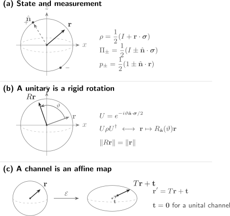
The Bloch representation organizes three one-qubit tasks. A projective measurement compares the state vector $\mathbf r$ with an axis $\hat{\mathbf n}$. A unitary rotates the ball rigidly, preserving radii and angles. A noisy channel acts affinely as $\mathbf r\mapsto T\mathbf r+\mathbf t$ and can contract, distort, or translate the accessible region. Not every affine map taking the ball into itself is automatically a completely positive quantum channel.

Measurement Axes

Projective measurement along an axis

For a unit vector $\hat{\mathbf n}$, the observable

$$\sigma_{\hat{\mathbf n}} = \hat{\mathbf n}\cdot\boldsymbol\sigma$$

has eigenvalues $\pm1$. Its projectors are

$$\Pi_\pm^{(\hat{\mathbf n})} = \frac12 \left( I\pm\hat{\mathbf n}\cdot\boldsymbol\sigma \right).$$

The Born rule gives

$$\begin{aligned} p_\pm &= \operatorname{Tr} \left( \rho\Pi_\pm^{(\hat{\mathbf n})} \right) \\ &= \frac12 \left( 1\pm\hat{\mathbf n}\cdot\mathbf r \right). \end{aligned}$$

The expectation value is the signed projection

$$\langle\sigma_{\hat{\mathbf n}}\rangle = p_+-p_- = \hat{\mathbf n}\cdot\mathbf r.$$

This is the operational meaning of the angle between the state and measurement vectors. Parallel pure-state and measurement axes give a certain $+1$ outcome; antiparallel axes give a certain $-1$ outcome; perpendicular axes give equal probabilities.

State axes and measurement axes are different objects

The same three-dimensional coordinates describe a state vector and a measurement direction, but they play different roles. The state belongs to the preparation model. The axis belongs to the measurement effect. If both are unknown, observed probabilities alone do not determine which one is miscalibrated.

A real detector may be biased or unsharp. A binary effect can be expanded as

$$E_+ = \alpha I+\mathbf m\cdot\boldsymbol\sigma,$$

with positivity constraints on $\alpha$ and $\mathbf m$. The resulting probability

$$p(+|\rho) = \alpha+\mathbf m\cdot\mathbf r$$

need not correspond to an ideal projective axis. Measurement Tomography owns reconstruction of unknown detector effects.

One-Qubit State Tomography

If ideal $X$, $Y$, and $Z$ measurements are calibrated, repeated outcomes estimate

$$\begin{aligned} r_x&=p_X(+)-p_X(-), \\ r_y&=p_Y(+)-p_Y(-), \\ r_z&=p_Z(+)-p_Z(-). \end{aligned}$$

For counts $N_{i,+}$ and $N_{i,-}$ in basis $i$,

$$\widehat r_i = \frac{N_{i,+}-N_{i,-}} {N_{i,+}+N_{i,-}}.$$

These estimates fluctuate. Independent linear inversion can produce

$$\lVert\widehat{\mathbf r}\rVert>1,$$

which corresponds to no positive density operator. This is not evidence for a state outside quantum mechanics; it is a sign that statistical noise and model assumptions must be handled. Constrained least squares, maximum likelihood, or Bayesian estimation can enforce physicality, but the estimator then has its own bias and uncertainty properties.

Tomography also inherits calibration error. If state preparation and measurement are both imperfect, a reconstructed vector can absorb errors from either side. A complete report states:

• the preparation and measurement model;
• shots per setting and uncertainty intervals;
• drift monitoring and data-selection rules;
• the estimator and positivity constraint;
• readout correction or calibration procedure;
• whether quoted fidelity is raw, corrected, or model dependent.

Three Pauli settings are informationally complete for one-qubit state tomography, but tomography scales poorly for many qubits. An arbitrary $n$-qubit density matrix has $4^n-1$ real parameters. The single-qubit sphere does not remove that scaling.

Rotations and Gates

Unitary gates rotate the ball

Ignoring an overall phase, every one-qubit unitary can be written

$$U(\hat{\mathbf n},\vartheta) = \exp \left( -\frac{i\vartheta}{2} \hat{\mathbf n}\cdot\boldsymbol\sigma \right).$$

Conjugation by $U$ maps

$$\rho' = U\rho U^\dagger$$

to a real-space rotation of the Bloch vector:

$$\mathbf r' = R_{\hat{\mathbf n}}(\vartheta)\mathbf r.$$

The rotation preserves

$$\lVert\mathbf r'\rVert = \lVert\mathbf r\rVert,$$

so a unitary cannot purify or mix an isolated qubit. It moves pure states along the surface and mixed states on a sphere of fixed radius.

The factor of $1/2$ in the exponential matters. A Bloch-vector rotation by angle $\vartheta$ is generated by $\vartheta\hat{\mathbf n}\cdot\boldsymbol\sigma/2$. The underlying spinor changes sign under a $2\pi$ rotation, while its density operator and Bloch vector return after $2\pi$. Spin Rotations owns the SU(2)-to-SO(3) derivation.

Familiar gates as rotations

Up to global phase:

Gate family	Bloch action
$X$	Rotation by $\pi$ about $x$
$Y$	Rotation by $\pi$ about $y$
$Z$	Rotation by $\pi$ about $z$
$R_x(\vartheta)$	Rotation by $\vartheta$ about $x$
$R_y(\vartheta)$	Rotation by $\vartheta$ about $y$
$R_z(\vartheta)$	Rotation by $\vartheta$ about $z$
$H$	Rotation by $\pi$ about $(\hat{\mathbf x}+\hat{\mathbf z})/\sqrt2$, up to phase

Single-Qubit Gates owns gate matrices, phase conventions, Euler decompositions, native controls, and compilation distinctions. Here the sphere provides the geometric action.

Schrödinger and Heisenberg pictures

One may rotate the state while holding the measurement axis fixed:

$$\mathbf r\mapsto R\mathbf r,$$

or hold the state fixed and rotate the observable oppositely:

$$\hat{\mathbf n}\mapsto R^{-1}\hat{\mathbf n}.$$

The probability is unchanged because

$$\hat{\mathbf n}\cdot R\mathbf r = \left( R^{-1}\hat{\mathbf n} \right)\cdot\mathbf r.$$

This distinction is practical. A laboratory may implement an $X$ measurement by applying a basis-change pulse and then using a fixed $Z$ readout. Whether the diagram shows a rotated state or rotated measurement axis depends on the chosen description.

Composition order

Rotations generally do not commute:

$$R_x(\alpha)R_y(\beta) \neq R_y(\beta)R_x(\alpha).$$

On a state column, the rightmost gate acts first. Bloch diagrams can hide this convention when arrows are drawn without an explicit time order. For pulse sequences, state the active rotation convention, axis orientation, and multiplication order.

Noisy Channels as Affine Maps

Every trace-preserving linear map on one-qubit operators acts affinely on the Bloch vector:

$$\mathbf r' = T\mathbf r+\mathbf t,$$

where $T$ is a real $3\times3$ matrix and $\mathbf t\in\mathbb R^3$. A physical quantum channel must be completely positive as well as trace preserving; this imposes constraints stronger than merely mapping the Bloch ball into itself.

A channel is unital when

$$\mathcal E(I)=I.$$

In Bloch coordinates this means

$$\mathbf t=\mathbf0.$$

Unital channels leave the center fixed, though they may contract or anisotropically distort the ball. Nonunital channels translate the center.

Dephasing

Define the dephasing family

$$\begin{aligned} \mathcal D_\lambda(\rho) &= \frac{1+\lambda}{2}\rho + \frac{1-\lambda}{2}Z\rho Z, \\ -1\leq\lambda\leq1. \end{aligned}$$

Its Bloch action is

$$(r_x,r_y,r_z) \longmapsto (\lambda r_x,\lambda r_y,r_z).$$

At $\lambda=0$, transverse coherence vanishes and the sphere collapses to the $z$-axis segment. Populations are unchanged. Negative $\lambda$ includes an additional phase inversion; in many dynamical dephasing models $\lambda$ decays from $1$ toward $0$. Dephasing Channel owns the Kraus, master-equation, and coherence-time treatments.

Depolarization

For the convention

$$\mathcal P_q(\rho) = (1-q)\rho+q\frac I2, \qquad 0\leq q\leq1,$$

the Bloch vector transforms isotropically:

$$\mathbf r\longmapsto(1-q)\mathbf r.$$

The ball contracts toward the center. Other sources use different depolarizing parameters, so the channel definition should accompany any quoted error probability.

Amplitude damping

With $|0\rangle$ chosen as the ground state and damping probability $\gamma$,

$$\begin{aligned} r_x'&=\sqrt{1-\gamma}\,r_x, \\ r_y'&=\sqrt{1-\gamma}\,r_y, \\ r_z'&=(1-\gamma)r_z+\gamma. \end{aligned}$$

This channel contracts and translates the ball toward $+z$. It is not unital because

$$\frac I2 \longmapsto \frac12 \left( I+\gamma Z \right).$$

Amplitude-Damping Channel gives the canonical channel derivation and physical interpretation.

A picture is not a complete process certification

Drawing an ellipsoid inside the ball is useful but insufficient to certify a channel. Complete positivity constrains the allowed contractions and translations, and correlated initial states can invalidate a state-independent reduced channel model. Process tomography additionally depends on trusted preparations and measurements. The Quantum Channels and Noise volume section owns Kraus, Choi, and Stinespring representations and their consistency conditions.

Geometric Diagnostics

Several one-qubit quantities become elementary functions of Bloch vectors.

Trace distance

For qubit states $\rho$ and $\sigma$ with vectors $\mathbf r$ and $\mathbf s$,

$$D(\rho,\sigma) = \frac12 \lVert\mathbf r-\mathbf s\rVert.$$

Thus optimal one-shot distinguishability is related to Euclidean separation in the ball. Antipodal pure states have distance $1$ and are orthogonal. The canonical definition and operational theorem are in Trace Distance.

Fidelity

Using the squared Uhlmann-fidelity convention,

$$\begin{aligned} F(\rho,\sigma) &= \frac{ 1+\mathbf r\cdot\mathbf s }{2} \\ &\quad + \frac{ \sqrt{1-\lVert\mathbf r\rVert^2} \sqrt{1-\lVert\mathbf s\rVert^2} }{2}. \end{aligned}$$

If $\rho=|\psi\rangle\langle\psi|$ is pure, this reduces to

$$F(\rho,\sigma) = \langle\psi|\sigma|\psi\rangle = \frac{1+\mathbf r\cdot\mathbf s}{2}.$$

Some sources call $\sqrt F$ the fidelity, so conventions must be stated. Fidelity fixes the site’s formula convention.

Entropy and radius

Because the eigenvalues are $(1\pm r)/2$ with $r=\lVert\mathbf r\rVert$, the von Neumann entropy is

$$S(\rho) = h_2 \left( \frac{1+r}{2} \right),$$

where $h_2$ is binary entropy. Entropy decreases monotonically from one bit at the center to zero on the surface. This simple radial dependence is special to one qubit.

Worked Operational Examples

Ramsey phase as azimuthal motion

Prepare $|0\rangle$, apply a $\pi/2$ pulse about $y$, and obtain the $+x$ state. A relative phase accumulation

$$U_\phi = \exp \left( -\frac{i\phi Z}{2} \right)$$

rotates the vector to

$$\mathbf r_\phi = (\cos\phi,\sin\phi,0).$$

An $X$ measurement gives

$$p_X(+|\phi) = \frac{1+\cos\phi}{2},$$

while a $Y$ measurement gives

$$p_Y(+|\phi) = \frac{1+\sin\phi}{2}.$$

The phase is invisible to a direct $Z$ measurement because $r_z=0$ throughout. This is why a final analysis pulse is needed to convert phase into a population difference.

Dephasing as loss of contrast

If the same equatorial state undergoes $\mathcal D_\lambda$,

$$\mathbf r_\phi \longmapsto \lambda (\cos\phi,\sin\phi,0).$$

Ramsey fringe contrast is multiplied by $\lambda$. The radial contraction summarizes the loss of coherence for this state family, but it does not by itself identify whether the cause was stochastic detuning, entanglement with an environment, averaging over drift, or another mechanism.

A calibrated measurement

Suppose a prepared state has

$$\mathbf r=(0.6,0,0.8),$$

which is pure because $\lVert\mathbf r\rVert=1$. Measuring along

$$\hat{\mathbf n} = \frac{ \hat{\mathbf x}+\hat{\mathbf z} }{\sqrt2}$$

gives

$$p_+ = \frac12 \left[ 1+\frac{1.4}{\sqrt2} \right] \approx0.995.$$

The near-certain outcome reflects geometric alignment, not simultaneous pre-existing $X$ and $Z$ values.

Limitations of the Picture

It is exact only for one qubit

An $n$-qubit density matrix requires $4^n-1$ real parameters. One may draw a reduced Bloch vector for each qubit, but those vectors omit correlations and entanglement. For the Bell state

$$|\Phi^+\rangle = \frac{|00\rangle+|11\rangle}{\sqrt2},$$

each qubit has $\mathbf r=\mathbf0$, yet the joint state is pure and maximally entangled. Two centered local balls do not describe the global state.

Generalized Bloch vectors are not ordinary balls

For a qudit, one can expand a state in $d^2-1$ traceless generators. Positivity does not fill a simple Euclidean ball when $d>2$. The elegant equivalence

$$\rho\geq0 \quad\Longleftrightarrow\quad \lVert\mathbf r\rVert\leq1$$

is special to $d=2$ under the standard normalization.

Axes require conventions and calibration

The $z$ axis usually names the computational basis, but whether $|0\rangle$ is north or south, ground or excited, horizontal or vertical polarization is conventional. Rotating-frame phases determine laboratory $x$ and $y$. A diagram without those conventions may reverse signs or rotation directions.

A trajectory does not identify a mechanism

The same visible path can arise from a Hamiltonian, a time-dependent control frame, postselection, or a noisy channel. A shrinking vector signals reduced one-qubit purity, but not a unique microscopic environment. Mechanistic claims require a declared dynamical model and independent tests.

A point is not an ensemble decomposition

Interior points do not reveal which classical mixture produced them. They may also be reduced states of entangled systems. The ball captures all one-qubit measurement statistics, not a hidden decomposition.

The sphere does not make noncommuting observables classical

The coordinates $r_x$, $r_y$, and $r_z$ are expectation values measurable on separate, similarly prepared systems. They are not three jointly readable values carried by one specimen. Uncertainty and measurement disturbance remain.

Common Mistakes

• Calling every point in the ball a pure state; only the surface is pure.
• Treating the Bloch vector as the state vector in $\mathbb C^2$.
• Forgetting that global phase is absent but relative phase sets the azimuth.
• Interpreting logical $x$, $y$, and $z$ as literal laboratory directions without an encoding map.
• Using $\mathbf r\mapsto T\mathbf r+\mathbf t$ without checking complete positivity.
• Inferring a calibrated state from data when the measurement axes are themselves unknown.
• Comparing depolarizing or dephasing parameters without checking conventions.
• Using local Bloch vectors as a complete description of a multi-qubit state.
• Treating linear-inversion estimates with $\lVert\widehat{\mathbf r}\rVert>1$ as physical states.
• Assuming a shrinking vector identifies one unique decoherence mechanism.

Exercises

1. Reconstruct a state from Pauli data

Ideal measurements give

$$\begin{aligned} p_X(+)&=0.65, \\ p_Y(+)&=0.30, \\ p_Z(+)&=0.75. \end{aligned}$$

Find the Bloch vector and density matrix. Is the estimate physical?

Solution

For a Pauli measurement,

$$r_i=2p_i(+)-1.$$

Therefore

$$\mathbf r=(0.30,-0.40,0.50).$$

Its length is

$$\begin{aligned} \lVert\mathbf r\rVert &= \sqrt{0.09+0.16+0.25} \\ &= \sqrt{0.50} <1, \end{aligned}$$

so it is physical. The density matrix is

$$\rho = \frac12 \begin{pmatrix} 1.50&0.30+0.40i \\ 0.30-0.40i&0.50 \end{pmatrix}.$$

Equivalently,

$$\rho = \begin{pmatrix} 0.75&0.15+0.20i \\ 0.15-0.20i&0.25 \end{pmatrix}.$$

2. Diagnose an unphysical linear estimate

Tomographic linear inversion gives

$$\widehat{\mathbf r}=(0.8,0.6,0.3).$$

Why is this not a valid qubit state, and what should an analyst do?

Solution

The squared length is

$$\lVert\widehat{\mathbf r}\rVert^2 = 0.8^2+0.6^2+0.3^2 = 1.09>1.$$

The smaller eigenvalue

$$\widehat\lambda_- = \frac{ 1-\sqrt{1.09} }{2}$$

is negative, so the reconstructed matrix is not positive semidefinite.

The analyst should not simply interpret the vector as “more than pure.” They should retain the raw counts, quantify statistical and calibration uncertainty, and use a documented physical estimator such as constrained least squares, maximum likelihood, or a Bayesian method. The choice of estimator and correction procedure must be reported.

3. Measure along a tilted axis

A qubit is in the $+x$ state, $\mathbf r=(1,0,0)$. It is measured along

$$\hat{\mathbf n} = \frac{ \hat{\mathbf x}+\hat{\mathbf z} }{\sqrt2}.$$

Find $p_+$ and $p_-$.

Solution

The dot product is

$$\hat{\mathbf n}\cdot\mathbf r = \frac1{\sqrt2}.$$

Hence

$$\begin{aligned} p_+ &= \frac12 \left( 1+\frac1{\sqrt2} \right), \\ p_- &= \frac12 \left( 1-\frac1{\sqrt2} \right). \end{aligned}$$

Numerically, $p_+\approx0.854$ and $p_-\approx0.146$.

4. Follow a gate rotation

The initial Bloch vector is $\mathbf r=(1,0,0)$. Apply

$$R_z\left(\frac\pi2\right) = \exp\left(-\frac{i\pi Z}{4}\right).$$

Find the final state and the probabilities of $X$, $Y$, and $Z$ outcomes.

Solution

A positive $\pi/2$ rotation about $z$ sends $+x$ to $+y$:

$$\mathbf r'=(0,1,0).$$

The final state is

$$|+i\rangle = \frac{|0\rangle+i|1\rangle}{\sqrt2}$$

up to global phase. Therefore

$$\begin{aligned} p_X(+)&=1/2, \\ p_Y(+)&=1, \\ p_Z(+)&=1/2. \end{aligned}$$

5. Dephasing and purity

The $+x$ state passes through $\mathcal D_\lambda$ with $0\leq\lambda\leq1$. Find its output Bloch vector and purity. Evaluate the result at $\lambda=0$ and $\lambda=1$.

Solution

The input vector is $(1,0,0)$, so

$$\mathbf r'=(\lambda,0,0).$$

Its purity is

$$\operatorname{Tr}(\rho'^2) = \frac{1+\lambda^2}{2}.$$

At $\lambda=1$, the state remains pure with purity $1$. At $\lambda=0$, the output is the center of the equatorial chord,

$$\rho'=\frac I2,$$

with purity $1/2$. Complete $Z$ dephasing of the equal superposition produces an equal incoherent mixture of $|0\rangle$ and $|1\rangle$.

6. Show that amplitude damping is nonunital

Apply amplitude damping with probability $\gamma$ to the maximally mixed state. Find the output vector and explain why the result proves the channel is nonunital.

Solution

The maximally mixed input has

$$\mathbf r=\mathbf0.$$

Using the affine map,

$$\mathbf r' = (0,0,\gamma).$$

Thus

$$\mathcal A_\gamma \left( \frac I2 \right) = \frac12 \left( I+\gamma Z \right).$$

For $\gamma>0$, this is not $I/2$. Equivalently,

$$\mathcal A_\gamma(I)\neq I.$$

The channel translates the center toward the ground-state pole and is nonunital.

Where to Go Next

• Information-Theoretic Foundations routes a one-qubit geometry question among carrier, state-validity, measurement, entropy, and resource owners before a specialized calculation begins.
• Bits, Qubits, Qudits, and Modes distinguishes the abstract qubit from its physical and logical realizations.
• Density Operators for Quantum Information extends the one-qubit picture to ensembles, reduced systems, instruments, state metrics, and numerical workflows.
• Bloch Sphere for Density Operators derives the ball, purity, and measurement formulas from density-operator structure.
• Bloch Sphere for Spin develops spinors, SU(2), SO(3), and physical spin directions.
• Bloch Sphere Geometry supplies the Pauli-coordinate mathematics.
• Pauli Matrices gives the matrix basis and algebra used throughout.
• BB84 uses the four states on the $z$ and $x$ axes as a prepare-and-measure key-distribution alphabet.
• Quantum Channels and Noise develops completely positive maps beyond the affine picture.
• Dephasing Channel and Amplitude-Damping Channel give canonical noise models.
• Measurement Tomography treats the inverse problem in which detector effects, rather than the input state, are unknown.
• State Tomography develops the statistical reconstruction workflow, physical estimators, uncertainty, SPAM limits, and many-qubit scaling beyond the geometric one-qubit example.
• Quantum Information Roadmap places states, gates, measurements, channels, and error correction in sequence.

References

• F. Bloch, “Nuclear induction,” Physical Review 70, 460–474, 1946, doi:10.1103/PhysRev.70.460.
• U. Fano, “Description of states in quantum mechanics by density matrix and operator techniques,” Reviews of Modern Physics 29, 74–93, 1957, doi:10.1103/RevModPhys.29.74.
• M. A. Nielsen and I. L. Chuang, Quantum Computation and Quantum Information, 10th anniversary ed., Cambridge University Press, 2010, doi:10.1017/CBO9780511976667.
• J. Watrous, The Theory of Quantum Information, Cambridge University Press, 2018, doi:10.1017/9781316848142.
• I. Bengtsson and K. Życzkowski, Geometry of Quantum States, 2nd ed., Cambridge University Press, 2017, doi:10.1017/9781139207010.
• J. Preskill, Lecture Notes for Physics 219/Computer Science 219: Quantum Computation, California Institute of Technology, course materials.
• D. F. V. James, P. G. Kwiat, W. J. Munro, and A. G. White, “Measurement of qubits,” Physical Review A 64, 052312, 2001, doi:10.1103/PhysRevA.64.052312.
• M. G. A. Paris and J. Řeháček, eds., Quantum State Estimation, Springer, 2004, doi:10.1007/b98673.
• M. B. Ruskai, S. Szarek, and E. Werner, “An analysis of completely-positive trace-preserving maps on $M_2$,” Linear Algebra and its Applications 347, 159–187, 2002, doi:10.1016/S0024-3795(01)00547-X.
• A. Fujiwara and P. Algoet, “One-to-one parametrization of quantum channels,” Physical Review A 59, 3290–3294, 1999, doi:10.1103/PhysRevA.59.3290.
• A. Gilchrist, N. K. Langford, and M. A. Nielsen, “Distance measures to compare real and ideal quantum processes,” Physical Review A 71, 062310, 2005, doi:10.1103/PhysRevA.71.062310.
• R. Blume-Kohout, “Optimal, reliable estimation of quantum states,” New Journal of Physics 12, 043034, 2010, doi:10.1088/1367-2630/12/4/043034.
• S. T. Merkel, J. M. Gambetta, J. A. Smolin, S. Poletto, A. D. Córcoles, B. R. Johnson, C. A. Ryan, and M. Steffen, “Self-consistent quantum process tomography,” Physical Review A 87, 062119, 2013, doi:10.1103/PhysRevA.87.062119.

Summary

The Bloch ball gives an exact operational coordinate system for one qubit. A state is represented by $\mathbf r=(\langle X\rangle,\langle Y\rangle,\langle Z\rangle)$ with $\lVert\mathbf r\rVert\leq1$; pure states lie on the surface, and mixed states lie inside. An ideal projective measurement along $\hat{\mathbf n}$ has probabilities $(1\pm\hat{\mathbf n}\cdot\mathbf r)/2$. Three calibrated Pauli measurements reconstruct the state, subject to finite-sample and calibration uncertainty.

One-qubit unitaries rotate the ball rigidly. General channels act affinely as $\mathbf r\mapsto T\mathbf r+\mathbf t$, with complete positivity constraining the allowed deformation. Dephasing contracts transverse components, depolarization contracts isotropically, and amplitude damping contracts and translates toward the ground-state pole. The picture is exact for one qubit but does not encode multi-qubit correlations, choose an ensemble decomposition, certify a channel, or replace calibration and uncertainty analysis.