State Tomography

Short Definition

Quantum state tomography infers a density operator from measurement outcomes obtained on many systems prepared by nominally the same procedure. It is an inverse problem with three indispensable ingredients:

1. a declared Hilbert space and state model;
2. a calibrated, informationally complete measurement design; and
3. a statistical estimator with an uncertainty statement.

For setting $s$ and outcome $a$, let $E_{a|s}$ be the modeled POVM effect. The Born probabilities are

$$p(a|s,\rho) = \operatorname{Tr}(\rho E_{a|s}), \qquad E_{a|s}\succeq 0, \qquad \sum_a E_{a|s}=I.$$

Tomography uses observed counts to solve this relation in reverse. It does not measure a wavefunction on one specimen, reveal an observer-independent ensemble decomposition, or eliminate assumptions about preparation and measurement. Rather, it estimates the state that best explains repeated data within the declared model.

This page is the canonical home for finite-dimensional state-reconstruction protocols, estimator choices, uncertainty, diagnostics, and scaling. Density Operators for Quantum Information owns the state object itself. POVMs owns generalized measurement theory, while Measurement Tomography owns reconstruction of unknown detectors. Optical homodyne inversion belongs with Homodyne and Heterodyne Detection. Process Tomography owns channel reconstruction. Shadow Tomography owns classical shadows as a targeted-observable alternative to full state reconstruction.

What the Data Mean

Suppose setting $s$ is used $N_s$ times and produces counts $n_{a|s}$, with

$$N_s=\sum_a n_{a|s}, \qquad f_{a|s}=\frac{n_{a|s}}{N_s}.$$

Under independent repetitions of one stationary preparation, the counts for each setting follow a multinomial model. Ignoring factors independent of $\rho$, the likelihood is

$$\mathcal L(\rho) = \prod_{s,a} \left[ \operatorname{Tr}(\rho E_{a|s}) \right]^{n_{a|s}},$$

and the log-likelihood is

$$\ell(\rho) = \sum_{s,a}n_{a|s} \log\!\left[ \operatorname{Tr}(\rho E_{a|s}) \right].$$

This compact expression contains most of tomography’s assumptions. The state must be repeatable enough for a common $\rho$ to make sense; the effects must describe the actual measurement; the recorded counts and setting choices must be accurate; and postselection must be part of the probability model rather than an undocumented edit.

The phrase “many copies” means many systems drawn from one preparation procedure, not repeated nondemolition access to every property of one system. Different settings generally consume different members of the ensemble because noncommuting observables cannot all be read from one ordinary copy.

Informational Completeness

Operator coordinates

Let the Hilbert-space dimension be $d$. Choose a Hermitian orthonormal operator basis $\{B_\mu\}_{\mu=0}^{d^2-1}$ satisfying

$$B_0=\frac{I}{\sqrt d}, \qquad \operatorname{Tr}(B_\mu B_\nu)=\delta_{\mu\nu}.$$

Every trace-one Hermitian operator can then be written as

$$\rho = \frac{I}{d} + \sum_{\mu=1}^{d^2-1}\theta_\mu B_\mu.$$

The probabilities are affine functions of the $d^2-1$ real coordinates:

$$p(a|s,\rho) = c_{a|s} + \sum_{\mu=1}^{d^2-1} A_{a|s,\mu}\theta_\mu,$$

where

$$c_{a|s}=\frac{\operatorname{Tr}E_{a|s}}{d}, \qquad A_{a|s,\mu}=\operatorname{Tr}(E_{a|s}B_\mu).$$

The design is informationally complete on the chosen model if no two allowed states give the same probabilities. For unrestricted $d$-dimensional states, this requires the centered design matrix to have rank

$$\operatorname{rank}A=d^2-1.$$

Equivalently, the measurement effects, together with the identity fixed by normalization, must span the Hermitian operator space. A single POVM therefore needs at least $d^2$ outcomes to be informationally complete. A laboratory may instead combine several projective settings. “One setting” and “one outcome” are different resources, so counts of them should not be compared casually.

Dual-frame reconstruction

If the setting $s$ is selected with known probability $w_s$, the joint effects

$$F_{s,a}=w_s E_{a|s}$$

form one POVM. For an informationally complete design there are dual operators $D_{s,a}$ such that every operator $X$ in the model space obeys

$$X = \sum_{s,a} \operatorname{Tr}(F_{s,a}X)D_{s,a}.$$

Replacing probabilities by joint empirical frequencies gives the linear inversion estimator

$$\widehat\rho_{\mathrm{LI}} = \sum_{s,a}f_{s,a}D_{s,a}, \qquad f_{s,a}=\frac{n_{s,a}}{\sum_{t,b}n_{t,b}}.$$

Under the exact sampling model, this estimator is linear and unbiased. Its weakness is equally important: finite-sample fluctuations can push it outside the convex set of density operators, producing a negative eigenvalue. That is not an exotic quantum state. It is a diagnostic that empirical frequencies do not lie exactly on the physical probability model.

Conditioning matters

Full rank is only an identifiability test. If the smallest singular value of the design matrix is tiny, inversion amplifies modest frequency errors into large coordinate errors. Schematically,

$$\delta\boldsymbol\theta = A^+\delta\mathbf f, \qquad \|\delta\boldsymbol\theta\|_2 \leq \|A^+\|_2\,\|\delta\mathbf f\|_2,$$

where $A^+$ is the pseudoinverse. The Singular Value Decomposition makes this noise amplification explicit. Symmetric and overcomplete designs can improve isotropy, robustness, and diagnostics even when a minimal design is formally sufficient.

Qubit Tomography

For one qubit,

$$\rho = \frac12 \left( I+r_xX+r_yY+r_zZ \right), \qquad \|\mathbf r\|_2\leq 1.$$

Ideal measurements along the three Pauli axes give

$$r_j = p_j(+)-p_j(-) = 2p_j(+)-1, \qquad j\in\{x,y,z\}.$$

Suppose $1{,}000$ shots per axis produce $730$, $610$, and $845$ positive outcomes for $X$, $Y$, and $Z$. Linear inversion gives

$$\widehat{\mathbf r} = (0.46,0.22,0.69), \qquad \|\widehat{\mathbf r}\|_2 \approx 0.858,$$

and hence

$$\widehat\rho = \begin{pmatrix} 0.845 & 0.23-0.11i\\ 0.23+0.11i & 0.155 \end{pmatrix}.$$

Its eigenvalues are approximately $0.929$ and $0.071$, so this particular linear estimate is physical. The estimated purity is

$$\operatorname{Tr}(\widehat\rho^2) = \frac{1+\|\widehat{\mathbf r}\|_2^2}{2} \approx 0.868.$$

These are point estimates, not exact properties. Under the ideal independent binomial model, the approximate standard error of each Bloch component is

$$\operatorname{se}(\widehat r_j) \approx \sqrt{\frac{1-\widehat r_j^2}{N_j}}.$$

For the data above, these are about $0.028$, $0.031$, and $0.023$. Calibration uncertainty, drift, and estimator-induced correlations are absent from those numbers.

The Bloch Sphere for Quantum Information develops the geometry and one-qubit conventions in more detail. Tomography is where that geometry becomes a statistical inverse problem.

Many-Qubit Pauli Tomography

For $n$ qubits, Pauli strings form an orthogonal operator basis:

$$\mathcal P_n = \{I,X,Y,Z\}^{\otimes n}, \qquad \operatorname{Tr}(PQ)=2^n\delta_{P,Q}.$$

The state expansion is

$$\rho = \frac{1}{2^n} \sum_{P\in\mathcal P_n} r_P P, \qquad r_P=\operatorname{Tr}(\rho P).$$

Normalization fixes $r_{I^{\otimes n}}=1$, leaving

$$4^n-1$$

independent real coordinates. Local Pauli tomography is often organized into $3^n$ tensor-product basis settings. Each setting has $2^n$ outcomes and simultaneously estimates several commuting Pauli strings through marginal products. This reuse is valuable, but both the number of generic state parameters and the conventional setting count remain exponential.

The raw outcome distribution should be retained. Reducing each setting immediately to selected expectation values can discard covariance information, hide leakage or normalization failures, and make later likelihood analysis impossible.

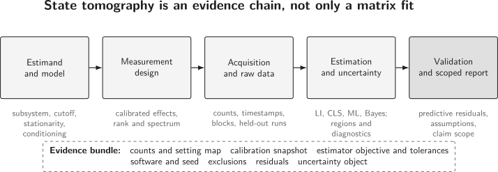
A defensible reconstruction is a chain of evidence. Physicality of $\widehat\rho$ is one check within that chain, not a substitute for measurement calibration, predictive validation, or uncertainty quantification.

Reconstruction Methods

Linear inversion and least squares

In coordinate form, ordinary least squares solves

$$\widehat{\boldsymbol\theta}_{\mathrm{LS}} = \underset{\boldsymbol\theta}{\operatorname{argmin}} \left\| W^{1/2} (A\boldsymbol\theta+\mathbf c-\mathbf f) \right\|_2^2,$$

where $W$ may account for unequal shot allocations or approximate frequency variances. With no positivity constraint, least squares and dual-frame inversion are closely related. They are fast, transparent, and useful for residual analysis. They can nevertheless return an operator with $\widehat\rho\not\succeq0$.

One can instead solve the constrained problem

$$\begin{aligned} \widehat\rho_{\mathrm{CLS}} ={}& \underset{\rho}{\operatorname{argmin}} \sum_{s,a}w_{a|s} \left[ f_{a|s}-\operatorname{Tr}(\rho E_{a|s}) \right]^2, \\ &\rho\succeq0, \qquad \operatorname{Tr}\rho=1. \end{aligned}$$

This is a convex optimization problem for fixed nonnegative weights. Projecting an unconstrained estimate onto the state set is another possibility, but the answer depends on the chosen norm and weights. “Clip negative eigenvalues and renormalize” silently defines an estimator; it is not a neutral cleanup step.

Maximum likelihood

The maximum-likelihood estimator is

$$\widehat\rho_{\mathrm{ML}} = \underset{\rho\succeq0,\,\operatorname{Tr}\rho=1} {\operatorname{argmax}} \sum_{s,a}n_{a|s} \log\operatorname{Tr}(\rho E_{a|s}).$$

Because the logarithm is concave and the probability is affine in $\rho$, the objective is concave on the convex state set. Direct semidefinite formulations therefore expose useful global structure. A parameterization such as

$$\rho(T)=\frac{TT^\dagger}{\operatorname{Tr}(TT^\dagger)}$$

guarantees physicality but can turn the numerical problem into a redundant, nonlinear parameter search. Convergence tolerances, zero-probability handling, and optimizer diagnostics belong in the reported method.

Maximum likelihood is not automatically unbiased, and finite data often place its solution on the boundary with one or more zero eigenvalues. If the design is incomplete, the likelihood may have a whole plateau of equally likely states. A secondary rule such as maximum entropy then adds information not contained in the observations and must be declared.

Bayesian estimation

A Bayesian analysis places a prior density $\pi(\rho)$ on the state space and updates it by

$$\pi(\rho|D) = \frac{\mathcal L(D|\rho)\pi(\rho)} {\int \mathcal L(D|\sigma)\pi(\sigma)\,d\sigma}.$$

The posterior mean

$$\widehat\rho_{\mathrm{BME}} = \int \rho\,\pi(\rho|D)\,d\rho$$

is physical and averages over state uncertainty. It is not prior-free. “Uniform over states” is incomplete until one specifies a measure or construction, and different priors can matter strongly for small data sets and nearly pure states. Bayesian state tomography should also not be confused with the real-time conditional dynamics developed in Bayesian Quantum Measurement.

No estimator dominates every task

Linear estimators preserve simple expectation identities but can be nonphysical. Constrained estimators respect the state space but introduce bias, especially near its boundary. Bayesian estimators integrate uncertainty but expose a prior choice and can be computationally demanding. An estimator should be selected against a declared loss function, state class, sample size, and downstream quantity, not by the visual smoothness of its density matrix.

Physicality Is Not Validation

Consider a one-qubit linear estimate

$$\widehat{\mathbf r}_{\mathrm{LI}} = (0.82,0.58,0.42).$$

Its length is approximately $1.089$, so the eigenvalues of the corresponding trace-one Hermitian matrix are

$$\lambda_\pm = \frac{1\pm\|\widehat{\mathbf r}_{\mathrm{LI}}\|_2}{2} \approx (1.044,-0.044).$$

For isotropic unweighted Euclidean loss, the nearest point in the Bloch ball is obtained by radial projection,

$$\widehat{\mathbf r}_{\mathrm{proj}} = \frac{\widehat{\mathbf r}_{\mathrm{LI}}} {\|\widehat{\mathbf r}_{\mathrm{LI}}\|_2}.$$

That estimate is physical, but the projection neither proves the measurement model nor explains why the frequencies were inconsistent. With unequal shot noise, correlated data, or anisotropic calibration uncertainty, radial projection is not even the relevant weighted solution.

A physical estimator can fit the wrong model beautifully. A wrong readout matrix, omitted leakage level, drifting source, or outcome-dependent loss may all be absorbed into a plausible $\widehat\rho$. Validation must therefore ask whether the fitted model predicts observations that were not used merely to force physicality.

Uncertainty and Error Regions

Local covariance

For regular interior models, the classical Fisher information of the tomographic experiment is

$$I_{\mu\nu}(\boldsymbol\theta) = \sum_s N_s\sum_a \frac{1}{p(a|s,\boldsymbol\theta)} \frac{\partial p(a|s,\boldsymbol\theta)}{\partial\theta_\mu} \frac{\partial p(a|s,\boldsymbol\theta)}{\partial\theta_\nu}.$$

Its inverse provides an asymptotic covariance benchmark when the usual regularity assumptions hold. The Fisher Information page develops that logic. Pure and nearly pure states sit near the boundary of state space, where Gaussian approximations, unconstrained coordinates, and standard likelihood-ratio rules can fail or converge slowly.

Confidence and credible regions

A frequentist confidence-region procedure $C(D)$ with level $1-\alpha$ aims to satisfy

$$\Pr_\rho\!\left[\rho\in C(D)\right] \geq 1-\alpha$$

for every state in the stated model. The probability is over repeated data, not a posterior probability assigned to the already fixed true state. A Bayesian credible region instead contains a chosen fraction of posterior mass and is conditional on the prior and likelihood. Both can be useful; they answer different questions.

Error bars should match the reported claim. A region for matrix entries does not immediately become a valid interval for fidelity, entropy, negativity, or the smallest eigenvalue. These are nonlinear functions, often most sensitive near a boundary. Propagate uncertainty through the actual quantity, or optimize that quantity over a justified state region.

Resampling

A parametric bootstrap simulates synthetic counts from a fitted state and the measurement model, reruns the complete estimator, and examines the resulting distribution. It can reveal estimator bias and non-Gaussian behavior, but its coverage inherits the fitted model and simulation assumptions. A nonparametric bootstrap assumes the empirical sample structure represents future sampling; naive resampling is unreliable when shots are correlated, settings drift, or blocks are not exchangeable.

Report the resampling unit. If calibration and science runs occur in blocks, resampling individual shots destroys block-level variation and usually makes the uncertainty look too small.

The Trusted-Measurement Problem

State tomography normally treats $E_{a|s}$ as known. If the actual effects are

$$E_{a|s}^{\mathrm{act}} = E_{a|s}^{\mathrm{nom}}+\Delta E_{a|s},$$

then, to first order,

$$\Delta p_{a|s} \approx \operatorname{Tr}(\Delta\rho\,E_{a|s}^{\mathrm{nom}}) + \operatorname{Tr}(\rho\,\Delta E_{a|s}).$$

The same probability discrepancy can therefore be attributed to the state, the detector, or both. Prepare-and-measure data constrain a bilinear pairing; they do not generally identify both factors without trusted references, structural assumptions, or additional operations. This is the state-tomography form of the SPAM problem discussed in Why Benchmarking Is Hard.

For a simple example, suppose a $Z$ readout flips either binary result with probability $\epsilon$. The measured contrast is

$$m_{\mathrm{obs}} = (1-2\epsilon)r_z.$$

Without independent knowledge of $\epsilon$, the observation does not separate readout contrast from state polarization. If $\epsilon$ is calibrated, inversion divides by $1-2\epsilon$ and amplifies both counting and calibration uncertainty.

Detector calibration is not a magic external truth source; it is another experiment with its own probe assumptions. The canonical dual problem is developed in Measurement Tomography. Joint or self-consistent methods can move the trust boundary, but they must state their remaining gauge freedoms and assumptions.

SPAM Errors owns the operational preparation–measurement ambiguity, assignment license, trusted-reference and self-consistent alternatives, gauge limits, context transfer, and mitigation boundary; this page retains state-reconstruction designs, estimators, uncertainty, validation, and scaling limits.

Drift, Correlations, and Model Mismatch

If shot $k$ is prepared in state $\rho_k$ while the measurement remains fixed, the average probability is

$$\overline p(a|s) = \frac1N\sum_{k=1}^N \operatorname{Tr}(\rho_kE_{a|s}) = \operatorname{Tr}(\overline\rho E_{a|s}),$$

with

$$\overline\rho=\frac1N\sum_{k=1}^N\rho_k.$$

Ordinary tomography may therefore reconstruct the time-averaged state even when no individual block was prepared in that state. If a source alternates between $|0\rangle$ and $|1\rangle$, aggregated data can look like the stationary mixed state $I/2$. Time tags or interleaved repeated settings are needed to distinguish these stories.

Correlations also invalidate multinomial variance formulas. Slow drift often creates overdispersion, while feedback or alternating sequences can create more structured residuals. Randomizing setting order, preserving timestamps, interleaving references, and analyzing blocks make these failures visible.

Other important model mismatches include:

• Leakage: population occupies levels outside the declared $d$-dimensional model.
• Loss and postselection: the reported state is conditional on survival or acceptance, possibly in an outcome-dependent way.
• Mislabeling: basis, qubit-order, endian, or phase conventions differ between acquisition and reconstruction.
• Context dependence: an effect calibrated alone changes when neighboring controls or simultaneous readout are active.
• Insufficient rank: the design is not informationally complete on the actual model, even if it is complete on the intended subspace.

Validation Before Interpretation

A useful protocol withholds some data or repeats nominally redundant settings. After fitting $\widehat\rho$, compare observed and predicted counts. One possible diagnostic is the multinomial deviance

$$G^2 = 2\sum_{s,a} n_{a|s} \log \frac{n_{a|s}} {N_s\operatorname{Tr}(\widehat\rho E_{a|s})},$$

where terms with $n_{a|s}=0$ are defined as zero. Its reference distribution must respect fitted constraints, finite counts, and boundary effects; a naive chi-square threshold is not universally valid. Calibrated simulations or held-out predictive checks are often safer.

Residuals should also be plotted against time, setting, outcome, qubit subset, and acquisition block. A small global average can conceal one basis with a large coherent mismatch. Reconstructing subsets of the data can test whether the supposed state is stable.

Tomography should answer a prior scientific question. If the claim concerns one target fidelity, witness, stabilizer set, or local correlator, full state reconstruction may be unnecessary and statistically wasteful. Direct estimation can also avoid the bias introduced by passing a linear observable through a nonlinear physical-state estimator.

Why Full Tomography Does Not Scale

For $n$ qubits, $d=2^n$ and an unrestricted density operator has

$$d^2-1=4^n-1$$

real parameters. Merely storing a dense estimate requires order $d^2$ numbers. Generic informational completeness, data acquisition, optimization, and uncertainty representation all inherit exponential growth.

There is no single “tomography complexity” because several resources differ:

• parameters describe the model dimension;
• settings count distinct control configurations;
• outcomes determine each setting’s probability simplex;
• copies or shots control statistical precision;
• measurement locality distinguishes product from collective protocols;
• classical cost covers storage, optimization, and uncertainty analysis.

For rank-$r$ states, ideal collective-measurement results can approach copy complexity of order

$$N = \widetilde O\!\left( \frac{dr}{\epsilon^2} \right)$$

for trace-distance error $\epsilon$, where the tilde hides logarithmic factors. The attainable rates and lower bounds change with the loss function and with whether collective or independent measurements are allowed. Such information- theoretic results should not be quoted as turnkey laboratory costs.

Additional structure can help:

• low-rank compressed sensing reduces measurements under suitable random-design and approximation assumptions;
• matrix-product or local reconstruction exploits restricted correlation and entanglement structure;
• permutation symmetry reduces the model for symmetric preparations;
• direct witnesses estimate a property without reconstructing every entry;
• classical shadows estimate many specified observables without delivering a uniformly accurate full density matrix.

These methods trade unrestricted reconstruction for assumptions or narrower questions. Positivity alone does not erase exponential worst-case complexity.

A Defensible Workflow

1. Define the estimand. State the subsystem, Hilbert-space cutoff, reference frame, time window, conditioning events, and whether the target is a full state or a particular functional.
2. Declare the measurement model. Record POVM effects, calibration data, setting probabilities, control circuits, readout corrections, and their uncertainties.
3. Check identifiability and conditioning. Compute the design rank and singular spectrum on the actual model space before collecting a large data set.
4. Design the acquisition. Randomize or interleave settings, preserve raw counts and timestamps, allocate held-out checks, and define exclusions in advance.
5. Fit more than one transparent estimator when useful. Comparing linear, constrained, and likelihood fits can expose boundary sensitivity; it does not replace a principled primary estimator.
6. Quantify uncertainty. Match confidence or credible regions to the reported metric and include calibration and block variation where possible.
7. Validate predictions. Inspect held-out counts, residuals, drift, leakage, and repeated settings before interpreting fidelity or entanglement.
8. Publish the evidence chain. Preserve raw counts, settings, calibration snapshots, estimator objective, constraints, software versions, random seeds, and analysis outputs. Reproducible Notebooks gives the broader artifact contract.

What a Tomographic Claim Should Say

A concise defensible result identifies:

• the preparation and acquisition epoch;
• the reconstructed subsystem and any truncation;
• the trusted measurement model and calibration source;
• the settings, outcomes, accepted shots, and exclusions;
• the primary estimator and numerical convergence checks;
• the uncertainty method and confidence or credibility level;
• predictive or residual diagnostics;
• the distance, fidelity convention, witness, or other reported functional;
• sensitivity to plausible SPAM, drift, and estimator alternatives.

“Tomography gives fidelity $0.99$” is incomplete. Fidelity to which target, under which convention, using which estimator, with what interval, and conditional on which measurement model are part of the scientific statement.

Common Mistakes

Treating frequencies as exact probabilities

Finite counts fluctuate. Matrix entries inferred from them require uncertainty, especially when nonlinear quantities are reported.

Calling a nonphysical linear estimate a new state

Negative eigenvalues usually diagnose sampling noise or model mismatch. They do not represent probabilities below zero.

Calling positivity a goodness-of-fit test

Constrained estimators are designed to return physical matrices even when the measurement model is wrong.

Assuming maximum likelihood is unbiased

The positivity boundary can bias eigenvalues, fidelities, and entanglement estimates. Bias depends on state, sample size, design, and reported functional.

Ignoring the measurement trust boundary

Nominal projectors are not calibrated POVM effects. Unmodeled readout error is typically absorbed into the reconstructed state.

Mixing settings, shots, and parameters

A protocol with few settings can still use many outcomes, copies, collective operations, or substantial classical processing.

Reporting only a density-matrix heat map

A plot without raw counts, uncertainty, conventions, and validation is an illustration, not a reproducible inference.

Reconstructing everything when the question is narrow

Full tomography can spend exponentially many resources to estimate quantities that a direct measurement would determine more accurately.

Exercises

Exercise 1: Count the identifiable directions

Show that a $d$-dimensional density operator has $d^2-1$ real degrees of freedom. Explain why a POVM with $m<d^2$ outcomes cannot be informationally complete for arbitrary states.

Solution

A Hermitian $d\times d$ matrix has $d$ real diagonal entries and $d(d-1)/2$ complex off-diagonal entries, for

$$d+2\frac{d(d-1)}2=d^2$$

real parameters. The trace-one condition removes one affine degree of freedom, leaving $d^2-1$. Positivity restricts the allowed region but does not reduce its interior dimension.

An $m$-outcome probability distribution has only $m-1$ independent numbers because its probabilities sum to one. Therefore $m-1\geq d^2-1$, or $m\geq d^2$, is necessary for one POVM to identify every state. It is not sufficient unless the effects span the operator space.

Exercise 2: Reconstruct the worked qubit

Using the $X$, $Y$, and $Z$ counts in the worked example, derive the density matrix, its eigenvalues, and its purity.

Solution

For $N=1000$ and positive counts $(730,610,845)$,

$$\widehat{\mathbf r} = 2(0.730,0.610,0.845)-(1,1,1) = (0.46,0.22,0.69).$$

Substituting in $\rho=(I+\mathbf r\cdot\boldsymbol\sigma)/2$ gives

$$\widehat\rho = \begin{pmatrix} (1+0.69)/2 & (0.46-0.22i)/2\\ (0.46+0.22i)/2 & (1-0.69)/2 \end{pmatrix}.$$

For a qubit, the eigenvalues are $(1\pm\|\mathbf r\|_2)/2$. Since $\|\mathbf r\|_2=\sqrt{0.7361}\approx0.858$, they are approximately $0.929$ and $0.071$. Finally,

$$\operatorname{Tr}(\widehat\rho^2) = \frac{1+0.7361}{2} = 0.86805.$$

Exercise 3: Diagnose and project an unphysical estimate

For $\widehat{\mathbf r}=(0.82,0.58,0.42)$, compute the negative eigenvalue and the isotropic Euclidean projection onto the Bloch ball. Why is this projection not a universal correction?

Solution

The length is

$$R = \sqrt{0.82^2+0.58^2+0.42^2} = \sqrt{1.1852} \approx1.089.$$

Thus $\lambda_-=(1-R)/2\approx-0.044$. The radial projection is

$$\mathbf r_{\mathrm{proj}} = \frac1{1.089}(0.82,0.58,0.42) \approx (0.753,0.533,0.386).$$

It is the nearest Bloch vector only for the stated isotropic Euclidean loss. Different variances, correlations, likelihoods, calibration uncertainties, or scientific loss functions define different estimators. Projection also cannot diagnose a wrong measurement model.

Exercise 4: Qubit tetrahedral tomography

Let four unit vectors $\mathbf n_k$ satisfy

$$\sum_{k=1}^4\mathbf n_k=0, \qquad \mathbf n_j\cdot\mathbf n_k=-\frac13 \quad(j\ne k),$$

and define

$$E_k=\frac14(I+\mathbf n_k\cdot\boldsymbol\sigma).$$

Show that $\{E_k\}$ is an informationally complete POVM and derive $\mathbf r$ from its probabilities $p_k$.

Solution

Each $E_k$ is positive because $I+\mathbf n_k\cdot\boldsymbol\sigma$ has eigenvalues $2$ and $0$. The vector sum condition gives

$$\sum_kE_k=I.$$

For $\rho=(I+\mathbf r\cdot\boldsymbol\sigma)/2$,

$$p_k = \operatorname{Tr}(\rho E_k) = \frac14(1+\mathbf n_k\cdot\mathbf r).$$

Tetrahedral symmetry implies

$$\sum_k\mathbf n_k\mathbf n_k^{\mathsf T} = \frac43 I_3.$$

Therefore

$$\sum_kp_k\mathbf n_k = \frac14\sum_k \mathbf n_k(\mathbf n_k\cdot\mathbf r) = \frac13\mathbf r,$$

so

$$\mathbf r=3\sum_kp_k\mathbf n_k.$$

The probabilities determine all three Bloch coordinates, proving informational completeness.

Exercise 5: Concavity of the log-likelihood

For a Hermitian trace-zero direction $\Delta$, show that the second directional derivative of the multinomial log-likelihood is nonpositive wherever all observed-event probabilities are positive.

Solution

Along $\rho(t)=\rho+t\Delta$,

$$\frac{d}{dt}\ell(\rho(t)) = \sum_{s,a}n_{a|s} \frac{\operatorname{Tr}(\Delta E_{a|s})} {\operatorname{Tr}(\rho(t)E_{a|s})}.$$

Differentiating again gives

$$\frac{d^2}{dt^2}\ell(\rho(t)) = -\sum_{s,a}n_{a|s} \frac{[\operatorname{Tr}(\Delta E_{a|s})]^2} {[\operatorname{Tr}(\rho(t)E_{a|s})]^2} \leq0.$$

Hence the log-likelihood is concave in $\rho$. Strict concavity, and therefore uniqueness, can fail when the data do not constrain some operator directions.

Exercise 6: Readout ambiguity and noise amplification

A binary detector flips either result with unknown probability $\epsilon$. Show that a measured $Z$ contrast does not identify both $r_z$ and $\epsilon$. If $\epsilon$ is known, find the corrected estimator and its variance in terms of the observed-contrast variance.

Solution

Symmetric flips map the ideal positive probability $p=(1+r_z)/2$ to

$$p_{\mathrm{obs}} = (1-\epsilon)p+\epsilon(1-p).$$

Thus

$$m_{\mathrm{obs}} = 2p_{\mathrm{obs}}-1 = (1-2\epsilon)r_z.$$

One observed number cannot determine two unknowns. If $\epsilon$ is known,

$$\widehat r_z = \frac{\widehat m_{\mathrm{obs}}}{1-2\epsilon}, \qquad \operatorname{Var}(\widehat r_z) = \frac{\operatorname{Var}(\widehat m_{\mathrm{obs}})} {(1-2\epsilon)^2}.$$

Calibration uncertainty in $\epsilon$ adds another propagated term. Correction therefore restores contrast only by amplifying uncertainty.

Exercise 7: A drifting source that looks mixed

A source alternates deterministically between $|0\rangle$ and $|1\rangle$. What state does aggregate tomography reconstruct if equal numbers of each are used? Give one acquisition change that exposes the drift.

Solution

The average state is

$$\overline\rho = \frac12|0\rangle\langle0| + \frac12|1\rangle\langle1| = \frac I2.$$

Because Born probabilities are linear in $\rho$, aggregate frequencies match the maximally mixed state. The data do not by themselves say that each shot was drawn independently from a stationary mixed preparation.

Preserving time order and comparing odd and even shots exposes the alternation. More generally, repeat each setting in interleaved time blocks and inspect blockwise estimates or residuals.

Exercise 8: Full reconstruction versus a targeted question

For eight qubits, compute the number of unrestricted real state parameters and the number of local Pauli basis settings. Compare a protocol using $1{,}000$ shots per setting with estimating only $\langle Z_1Z_2\rangle$ using the same shots.

Solution

The unrestricted parameter count is

$$4^8-1=65{,}535,$$

and the number of local $X/Y/Z$ basis settings is

$$3^8=6{,}561.$$

At $1{,}000$ shots per setting, conventional full acquisition uses $6{,}561{,}000$ shots, before calibration and repeats. The correlator $\langle Z_1Z_2\rangle$ can be estimated from one setting with $1{,}000$ shots; measurements of the other qubits may be marginalized. Full tomography answers far more questions, but it is wasteful when the scientific claim needs only that correlator.

Further Connections

• Density Operators for Quantum Information for positivity, purity, trace distance, fidelity, and reduced states.
• POVMs for effects, continuous outcomes, and informational completeness.
• Measurement Tomography for the dual inverse problem of reconstructing detector effects.
• Process Tomography for standard and ancilla-assisted reconstruction of channels under CP, trace, SPAM, and composability constraints.
• Shadow Tomography for reusable randomized-measurement snapshots, ensemble-dependent prediction costs, target-aware schedules, and noise-calibrated property estimation.
• Certification of Entanglement explains how confidence regions, PPT tests, and witness optimization convert finite tomographic data into a scoped entanglement claim.
• Bloch Sphere for Quantum Information for one-qubit geometry and Pauli-axis conventions.
• Why Benchmarking Is Hard for SPAM, context dependence, drift, and evidence contracts.
• Claims, Hype, and Evidence Standards for calibrating the strength of claims supported by a reconstruction.

References

1. D. F. V. James, P. G. Kwiat, W. J. Munro, and A. G. White, “Measurement of qubits,” Physical Review A 64, 052312 (2001), doi:10.1103/PhysRevA.64.052312.
2. Z. Hradil, “Quantum-state estimation,” Physical Review A 55, R1561–R1564 (1997), doi:10.1103/PhysRevA.55.R1561.
3. A. J. Scott, “Tight informationally complete quantum measurements,” Journal of Physics A: Mathematical and General 39, 13507–13530 (2006), doi:10.1088/0305-4470/39/43/009.
4. M. D. de Burgh, N. K. Langford, A. C. Doherty, and A. Gilchrist, “Choice of measurement sets in qubit tomography,” Physical Review A 78, 052122 (2008), doi:10.1103/PhysRevA.78.052122.
5. R. Blume-Kohout, “Optimal, reliable estimation of quantum states,” New Journal of Physics 12, 043034 (2010), doi:10.1088/1367-2630/12/4/043034.
6. J. A. Smolin, J. M. Gambetta, and G. Smith, “Efficient method for computing the maximum-likelihood quantum state from measurements with additive Gaussian noise,” Physical Review Letters 108, 070502 (2012), doi:10.1103/PhysRevLett.108.070502.
7. M. Christandl and R. Renner, “Reliable quantum state tomography,” Physical Review Letters 109, 120403 (2012), with erratum 159903, doi:10.1103/PhysRevLett.109.120403.
8. P. Faist and R. Renner, “Practical, reliable error bars in quantum tomography,” Physical Review Letters 117, 010404 (2016), doi:10.1103/PhysRevLett.117.010404.
9. C. Schwemmer et al., “Systematic errors in current quantum state tomography tools,” Physical Review Letters 114, 080403 (2015), doi:10.1103/PhysRevLett.114.080403.
10. D. Gross, Y.-K. Liu, S. T. Flammia, S. Becker, and J. Eisert, “Quantum state tomography via compressed sensing,” Physical Review Letters 105, 150401 (2010), doi:10.1103/PhysRevLett.105.150401.
11. J. Haah, A. W. Harrow, Z. Ji, X. Wu, and N. Yu, “Sample-optimal tomography of quantum states,” Proceedings of the 48th Annual ACM Symposium on Theory of Computing, 913–925 (2016), doi:10.1145/2897518.2897585.
12. D. H. Mahler et al., “Adaptive quantum state tomography improves accuracy quadratically,” Physical Review Letters 111, 183601 (2013), doi:10.1103/PhysRevLett.111.183601.
13. S. J. van Enk and R. Blume-Kohout, “When quantum tomography goes wrong: drift of quantum sources and other errors,” New Journal of Physics 15, 025024 (2013), doi:10.1088/1367-2630/15/2/025024.
14. M. Cramer et al., “Efficient quantum state tomography,” Nature Communications 1, 149 (2010), doi:10.1038/ncomms1147.

Summary

• State tomography estimates a repeatable preparation within a declared Hilbert space and trusted measurement model.
• Informational completeness requires sensitivity to all $d^2-1$ independent state directions; good conditioning is an additional requirement.
• Linear inversion is transparent but may be nonphysical. Constrained, likelihood, and Bayesian estimators impose different assumptions and biases.
• A physical point estimate is not a validation result. Reliable claims require uncertainty, residual checks, calibration provenance, and drift diagnostics.
• Full tomography scales exponentially for unrestricted many-qubit states. Structured or targeted methods gain efficiency by narrowing the state class or the scientific question.