Certification of Entanglement

Short Definition

Entanglement certification is the inference that experimental data are incompatible with a declared nonentangled model under a declared set of physical, device, and statistical assumptions. The conclusion is not merely that a reconstructed density matrix looks entangled. A certification claim must identify:

1. the systems and tensor-product partition;
2. the null class to be rejected;
3. which preparations and measurements are trusted;
4. how losses, postselection, drift, and memory are treated;
5. the finite-data rule used to control false certification.

For ordinary bipartite entanglement, the null class is the convex set of separable states

$$\mathcal S_{A:B} = \left\{ \sum_{\lambda} q_\lambda \rho_A^\lambda \otimes \rho_B^\lambda : q_\lambda\geq 0,\ \sum_\lambda q_\lambda=1 \right\}.$$

A certificate is evidence that the data could not have arisen from any member of $\mathcal S_{A:B}$ compatible with the stated measurement model. For multipartite experiments, the null set might instead be the biseparable states, the $k$-producible states, or states with Schmidt number at most $r$. Those choices support different conclusions.

Entanglement detection is generally one-sided. Passing a valid test proves entanglement within its scope; failing it usually proves nothing. There are entangled states that a chosen witness, finite Bell scenario, steering test, or incomplete measurement design does not detect.

Canonical Scope

This page owns the operational choice and audit of entanglement-certification protocols:

• trusted-device witnesses, tomography-based tests, and uncertainty margins;
• one-sided-device-independent steering tests;
• device-independent Bell certification and self-testing;
• multipartite, entanglement-depth, and dimensionality claims;
• finite statistics, drift, loss, postselection, and witness selection;
• the minimum evidence record needed for a defensible experimental claim.

Entanglement Witnesses owns witness geometry, positive maps, and the detailed Bell-state witness derivation. Negativity and PPT Criterion owns partial transposition and negativity. Multipartite Separability owns the mathematical hierarchy of multipartite separability classes.

CHSH Inequality owns the compact theorem and derivation, while Bell Inequality Experiments owns the historical experiments and foundational development. State Tomography owns density-matrix reconstruction. Here those results are used to answer a different question: what has an experiment certified, under which trust model, and with what error control? Network Verification applies that hierarchy to destructive sampling, independent sources, end-to-end routes, heralded channels, operational service thresholds, and possibly dishonest network nodes.

A Certificate Is a Rejected Null Model

Let $\mathcal N$ be the null class. It may encode separability as well as constraints on dimension, preparation drift, measurement calibration, or causal structure. Experimental records $D$ are converted into a test statistic $T(D)$ for which the null model supplies a bound

$$T(P) \leq \beta_{\mathcal N} \qquad \text{for every } P\in\mathcal N.$$

The data certify a departure from $\mathcal N$ only after finite-sample and systematic uncertainty are included. One possible decision rule is

$$T_{\mathrm{low}}(D;1-\alpha) > \beta_{\mathcal N},$$

where $T_{\mathrm{low}}$ is a valid one-sided lower confidence bound and $\alpha$ controls the probability of rejecting a true null under the specified analysis.

This formulation separates four statements that are often conflated:

statement	question answered
detection	do the data exclude the chosen nonentangled null?
characterization	which state, assemblage, or correlations best describe the data?
quantification	what lower or upper bound follows for an entanglement measure?
usefulness	is the certified resource sufficient for a named task?

A negative witness value detects entanglement but is not automatically an entanglement measure. A Bell violation detects nonlocal correlations but does not by itself give the singlet fidelity. A self-testing theorem can provide a fidelity bound, but only for the target and equivalence relation in that theorem.

Declare the physical partition

Entanglement is defined relative to a subsystem decomposition. A report must say what counts as $A$, $B$, and any additional parties. For identical particles, field modes, encoded logical qubits, or constrained Hilbert spaces, this declaration is substantive rather than typographical.

A state separable across one cut can be entangled across another:

$$\rho\in\mathcal S_{A:BC} \quad\not\Rightarrow\quad \rho\in\mathcal S_{AB:C}.$$

Likewise, pairwise entanglement, genuine multipartite entanglement, and entanglement depth are different targets. The certificate must name the one actually tested.

Trust Models

Entanglement certification forms a hierarchy according to how much is assumed about the measurement devices.

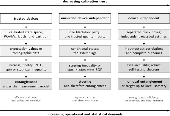
Moving right reduces calibration trust but increases the operational demands on isolation, setting randomness, detection efficiency, causal separation, and statistics. Device independence changes the assumptions; it does not remove assumptions.

Trusted devices

In a trusted-device protocol, the POVM elements, basis labels, subsystem map, and often the Hilbert-space dimension are treated as calibrated. The observed frequencies are interpreted through a quantum measurement model such as

$$p(a,b\mid x,y) = \operatorname{Tr} \left[ \rho_{AB} \left( M_{a\mid x}^{A} \otimes N_{b\mid y}^{B} \right) \right].$$

Witnesses, PPT tests applied to tomography, fidelity thresholds, stabilizer tests, spin-squeezing inequalities, and many randomized-measurement methods belong here. These tests can be highly efficient, but a calibration error can move the separable bound or bias the observed statistic.

One-sided device independence

In a steering experiment, one party’s measurement device is uncharacterized while the other party has trusted quantum measurements. For steering from Alice to Bob, Alice’s input $x$ and output $a$ are treated as black-box data; Bob trusts his local state space and measurements. A violation of a local hidden-state model certifies entanglement without trusting Alice’s measurement implementation.

Full device independence

In a device-independent Bell experiment, neither party’s measurement operators, state dimension, nor internal implementation is assumed. The certificate uses only the conditional input-output probabilities $p(a,b\mid x,y)$ plus causal and operational assumptions such as no communication during a trial and sufficiently independent setting choices. A Bell violation then certifies entanglement. With stronger rigidity results, the correlations can also self-test a target state and measurements up to unobservable local freedoms.

The logical nesting is

$$\text{Bell nonlocal} \subsetneq \text{steerable} \subsetneq \text{entangled}.$$

The inclusions are strict for mixed states. Consequently, increasing device independence normally reduces the set of states that a fixed experimental scenario can certify.

Trusted-Device Witnesses

An entanglement witness for null set $\mathcal N$ is a Hermitian observable $W$ satisfying

$$\operatorname{Tr}(W\sigma) \geq 0 \qquad \text{for all } \sigma\in\mathcal N,$$

while at least one target state obeys

$$\operatorname{Tr}(W\rho)<0.$$

For the Bell state

$$\lvert\Phi^+\rangle = \frac{ \lvert00\rangle+\lvert11\rangle }{ \sqrt2 },$$

a standard fidelity witness is

$$W_{\Phi^+} = \frac12 I - \lvert\Phi^+\rangle \langle\Phi^+\rvert.$$

Its expectation is negative exactly when the measured Bell-state fidelity exceeds $1/2$:

$$\langle W_{\Phi^+}\rangle_\rho = \frac12 - F_{\Phi^+}(\rho) <0.$$

The canonical witness page derives its Pauli decomposition and geometric meaning. Operationally, the important point is that the decomposition fixes the required measurement settings:

$$W_{\Phi^+} = \frac14 \left( I - X\otimes X + Y\otimes Y - Z\otimes Z \right).$$

A valid implementation therefore requires calibrated $X$, $Y$, and $Z$ measurements, a declared outcome convention, and a statistical analysis of the three correlators.

Witness efficiency and incompleteness

If

$$W=\sum_{j=1}^{m} c_j O_j,$$

then only the observables $O_j$ need be estimated. This can require far fewer settings than full tomography. The price is directional sensitivity: $W$ detects states on one side of one separating hyperplane. A nonnegative result means

$$\operatorname{Tr}(W\rho)\geq0,$$

not that $\rho$ is separable.

Witness choice should therefore follow the scientific target:

• fidelity witnesses are efficient near a known pure target;
• stabilizer witnesses exploit graph-state or code structure;
• collective-spin inequalities address large ensembles with limited access;
• Hamiltonian witnesses use an energy bound over separable states;
• Schmidt-number witnesses test entanglement dimensionality;
• genuine-multipartite witnesses use the biseparable set as their null.

The null bound must match the implemented observables. Substituting an approximate calibration into a witness optimized for ideal axes can invalidate the inequality.

Finite-Data Witness Certification

Suppose each trial $i$ produces a bounded score $Z_i$ whose conditional expectation is at least zero for every separable preparation allowed by the null:

$$\mathbb E_{\mathcal N} \left[ Z_i \mid \mathcal F_{i-1} \right] \geq 0.$$

The history $\mathcal F_{i-1}$ may include earlier settings and outcomes. This conditional formulation can accommodate source drift and memory that an i.i.d. error bar would miss.

For a simple bounded i.i.d. design, let

$$Z_i\in[z_{\min},z_{\max}], \qquad \widehat w = \frac1n \sum_{i=1}^{n} Z_i.$$

Hoeffding’s inequality gives the conservative one-sided statement

$$\Pr \left[ \mathbb E Z \leq \widehat w-\delta_\alpha \right] \leq \alpha,$$

with

$$\delta_\alpha = \left( z_{\max}-z_{\min} \right) \sqrt{ \frac{ \log(1/\alpha) }{ 2n } }.$$

If the separable bound is zero and negativity indicates entanglement, a corresponding upper confidence bound is

$$w_{\mathrm{up}} = \widehat w+\delta_\alpha.$$

Certification requires $w_{\mathrm{up}}<0$, not merely $\widehat w<0$. Tighter valid analyses can use empirical Bernstein bounds, likelihood ratios, confidence regions, martingales, or protocol-specific tests.

Separate random and systematic uncertainty

Let $b_{\mathrm{cal}}$ bound the worst-case upward shift needed to protect against measurement miscalibration and $b_{\mathrm{model}}$ cover other declared model uncertainty. A conservative decision uses

$$w_{\mathrm{cert}} = \widehat w + \delta_{\mathrm{stat}} + b_{\mathrm{cal}} + b_{\mathrm{model}}.$$

The claim is accepted only if

$$w_{\mathrm{cert}}<0.$$

More data can shrink $\delta_{\mathrm{stat}}$ but not an unresolved calibration bound. Reporting many standard deviations while ignoring a larger basis-angle error is not strong evidence.

For a witness decomposed over settings, shot allocation should reflect both coefficient magnitude and variance. If setting $j$ uses $n_j$ trials and single-shot variance $v_j$, then approximately

$$\operatorname{Var}(\widehat w) = \sum_j \frac{ c_j^2 v_j }{ n_j }.$$

Under a fixed total shot budget and known variances, the variance-minimizing allocation obeys

$$n_j \propto \lvert c_j\rvert \sqrt{v_j}.$$

Pilot estimates used for this allocation should be separated from confirmatory data or incorporated into a prespecified adaptive design.

Data-dependent witness selection

Optimizing $W$ on the same fluctuations later used to claim significance creates selection bias. Searching $K$ witnesses and reporting only the most negative one changes the null distribution. Defensible options include:

1. choose the witness from theory before data collection;
2. use training data to select $W$ and independent test data to evaluate it;
3. include the search in a simultaneous or multiple-testing correction;
4. use a confidence region that is valid for all selected functionals.

The same concern applies to choosing a partition, time window, qubit subset, postselection threshold, or Bell inequality after viewing the outcomes.

Tomography, PPT, and Convex Tests

Tomographically complete measurements can reconstruct an estimate $\widehat\rho$. One may then test whether the data are compatible with a separable state, apply the PPT criterion, or optimize a witness around the estimate. The inference must act on the likelihood or a valid confidence region, not only on a point estimate.

For partial transposition on subsystem $B$,

$$\rho^{T_B} = \sum_{i,j,k,l} \rho_{ij,kl} \lvert i,l\rangle \langle k,j\rvert.$$

Every separable state satisfies

$$\rho^{T_B}\succeq0.$$

Thus a statistically supported negative eigenvalue certifies entanglement. For $2\times2$ and $2\times3$ systems, PPT is also sufficient for separability. In higher dimensions, PPT-entangled states exist, so $\rho^{T_B}\succeq0$ does not certify separability.

The smallest eigenvalue of a reconstructed matrix is a nonlinear, boundary-sensitive statistic. Naive Gaussian propagation can be misleading near zero. Better options include likelihood-ratio tests against the PPT or separable set, bootstrap procedures whose validity has been established for the boundary problem, or confidence regions entirely contained in the NPT set.

Tomography is flexible but expensive. For $d$-dimensional states, an unconstrained density matrix has $d^2-1$ real parameters. This scaling, combined with difficult separability optimization, is why structured witnesses and randomized estimators are often preferred for large systems.

Measurement-Device-Independent Variants

There are intermediate protocols beyond the simple three-level hierarchy. In a measurement-device-independent entanglement witness, a referee supplies trusted quantum input states while the joint measurement devices are untrusted. The score is constructed so that every separable shared state obeys a bound regardless of the measurement implementation.

This removes some detector-calibration attacks but introduces trust in the quantum inputs and their independence. It is therefore neither the same as an ordinary calibrated witness nor automatically fully device independent. Reports should spell out which source, input channel, random generator, and measurement stations are trusted.

Steering Certification

For steering from Alice to Bob, Alice receives a classical setting $x$ and announces outcome $a$. Bob performs trusted tomography on his conditional subnormalized states. The resulting assemblage is

$$\sigma_{a\mid x}^{B} = \operatorname{Tr}_A \left[ \left( M_{a\mid x}^{A} \otimes I_B \right) \rho_{AB} \right].$$

It obeys

$$\sum_a \sigma_{a\mid x}^{B} = \rho_B \qquad \text{for every }x$$

when no signaling from Alice’s setting to Bob is present.

A local hidden-state model has the form

$$\sigma_{a\mid x}^{B} = \sum_\lambda p(\lambda) p(a\mid x,\lambda) \rho_\lambda^B.$$

Here Alice may use arbitrary classical response functions, but Bob’s systems are drawn from a pre-existing ensemble of quantum states. If no such decomposition is compatible with the assemblage, Alice steers Bob, and the shared state is entangled.

For finitely many settings and outcomes, testing the local hidden-state model can often be written as a semidefinite feasibility problem. Deterministic response functions $D(a\mid x,\lambda)$ suffice at the extremal points:

$$\begin{aligned} \text{find}\quad &\{\tau_\lambda\succeq0\},\\ \text{such that}\quad &\sigma_{a\mid x} = \sum_\lambda D(a\mid x,\lambda) \tau_\lambda. \end{aligned}$$

In finite data, equality is replaced by a likelihood or confidence-region constraint. A dual infeasibility certificate supplies a steering inequality of the form

$$\sum_{a,x} \operatorname{Tr} \left[ F_{a\mid x} \sigma_{a\mid x} \right] > \beta_{\mathrm{LHS}}.$$

What steering does and does not trust

Bob must trust:

• the dimension and calibration of his measured system;
• the correspondence between detector records and POVM outcomes;
• the completeness of Alice’s outcome alphabet, including no-click events;
• the trial definition and absence of forbidden communication into his lab.

Alice’s measurement operators need not be characterized. But Alice cannot silently discard inconvenient trials unless the inequality and loss model allow it. Steering is directional: a mixed state may be steerable from Alice to Bob but not from Bob to Alice under the same measurement class.

Bell Tests as Entanglement Certificates

In a bipartite Bell scenario, each trial has settings $x,y$ and outcomes $a,b$. A local hidden-variable model factorizes conditionally on shared classical information:

$$p(a,b\mid x,y) = \int d\lambda\, \mu(\lambda) p(a\mid x,\lambda) p(b\mid y,\lambda).$$

Every separable quantum state generates local correlations for local measurements. Therefore, a valid Bell violation certifies entanglement without trusting the internal state or measurement operators.

For binary observables $A_x,B_y\in\{-1,+1\}$, the CHSH expression is

$$S = \langle A_0B_0\rangle + \langle A_0B_1\rangle + \langle A_1B_0\rangle - \langle A_1B_1\rangle.$$

Local models obey

$$\lvert S\rvert\leq2,$$

whereas quantum theory allows

$$\lvert S\rvert\leq2\sqrt2.$$

The second bound is Tsirelson’s bound. The canonical CHSH entry derives both bounds. For certification, the crucial fact is

$$S_{\mathrm{low}}>2 \quad\Longrightarrow\quad \text{entanglement},$$

provided the Bell-test assumptions and finite-statistics analysis are valid.

Bell nonlocality is stronger than entanglement

No Bell violation from a particular state and measurement set does not imply separability. Some entangled mixed states admit local models for substantial measurement classes, and a finite experiment probes only selected settings. Bell tests are powerful because of their low device trust, not because they detect every entangled state efficiently.

Operational loopholes

A Bell certificate must address more than a numerical value of $S$:

issue	failure mode
locality	one station’s setting or outcome can influence the other during a trial
detection	discarded no-click events create a selected subensemble
setting independence	hidden variables correlate with setting choices
coincidence timing	the pairing rule selects events using outcomes or settings
memory	non-i.i.d. devices exploit past settings and outcomes
signaling	observed marginals depend on the distant setting beyond expected fluctuation
stopping	collection ends after a favorable fluctuation

Event-ready trial definitions, high-efficiency detection, spacelike separation, recorded random settings, complete outcome alphabets, and martingale or prediction-based statistical tests address these concerns. The 2015 loophole-free experiments showed that these requirements can be met, but they remain protocol requirements rather than inherited labels.

The null hypothesis for a Bell analysis should include the allowed memory and setting predictability. A valid $p$-value has the form

$$p_{\mathrm{Bell}} = \sup_{P\in\mathcal L} \Pr_P \left[ T(D)\geq T(D_{\mathrm{obs}}) \right],$$

where $\mathcal L$ is the declared class of local strategies. A Gaussian number-of-standard-deviations estimate is not automatically valid against adaptive local models.

Self-Testing

A Bell violation proves that the correlations are nonlocal. Self-testing asks a stronger inverse question: do those correlations identify a target state and measurements without looking inside the devices?

Exact self-testing never identifies an arbitrary laboratory tensor factor literally. Local basis changes, unused degrees of freedom, and relabelings cannot be observed from the correlations. The appropriate conclusion is that there exist local isometries $\Phi_A$ and $\Phi_B$ such that

$$\begin{aligned} & \left( \Phi_A\otimes\Phi_B \right) \rho_{AB} \left( \Phi_A\otimes\Phi_B \right)^\dagger\\ &\qquad = \rho_{\mathrm{junk}} \otimes \lvert\psi_{\mathrm{tar}}\rangle \langle\psi_{\mathrm{tar}}\rvert \end{aligned}$$

in the ideal case, with corresponding relations for the measured observables on the support of the state.

For maximal CHSH violation, the target can be a Bell pair with anticommuting qubit observables, up to these local freedoms. Real experiments require a robust statement. One common target is the extractability

$$\Xi(\rho\to\psi_{\mathrm{tar}}) = \max_{\Lambda_A,\Lambda_B} F \left[ \left( \Lambda_A\otimes\Lambda_B \right)(\rho), \psi_{\mathrm{tar}} \right],$$

where $\Lambda_A$ and $\Lambda_B$ are local extraction channels. A robust self-testing theorem gives

$$\Xi \geq f(S_{\mathrm{low}}),$$

for a rigorously derived function $f$. The observed violation, its confidence bound, and the theorem’s convention must all match.

Why robustness matters

Near an ideal extremal correlation, a small score deficit may map to a much larger uncertainty in state fidelity. Some analytic CHSH bounds become nontrivial only above a violation threshold. Different self-testing bounds can use different fidelity notions, dimensions, symmetry conventions, and noise assumptions. Quoting only the ideal statement at $S=2\sqrt2$ is not an experimental certificate.

Self-testing still assumes:

• the validity of quantum mechanics for the devices;
• distinct parties that cannot communicate during a trial;
• sufficiently independent and recorded setting choices;
• complete outcomes and a justified treatment of loss;
• a valid finite-data lower bound on the Bell score;
• the causal architecture required by the theorem.

It certifies a target up to local isometry, not the manufacturer’s qubit labels, chip layout, or microscopic Hamiltonian.

Multipartite Certification

For $N\geq3$ parties, the word entangled is underspecified. A state is biseparable if it is a mixture of states separable across possibly different bipartitions:

$$\rho_{\mathrm{bisep}} = \sum_{\lambda} q_\lambda \rho_{\lambda}^{S_\lambda} \otimes \rho_{\lambda}^{\bar S_\lambda}.$$

A state outside this convex set is genuinely multipartite entangled. Notice that the partition $S_\lambda:\bar S_\lambda$ may change with $\lambda$. Showing entanglement across every fixed cut separately does not always exclude a biseparable mixture unless the analysis treats the common data and mixture structure correctly.

A genuine-multipartite-entanglement witness satisfies

$$\operatorname{Tr} \left( W_{\mathrm{GME}} \sigma_{\mathrm{bisep}} \right) \geq0$$

for every biseparable state. For an $N$-qubit GHZ target,

$$\lvert\mathrm{GHZ}_N\rangle = \frac{ \lvert0\rangle^{\otimes N} + \lvert1\rangle^{\otimes N} }{ \sqrt2 },$$

the maximal biseparable fidelity is $1/2$. Thus

$$W_{\mathrm{GHZ}} = \frac12 I - \lvert\mathrm{GHZ}_N\rangle \langle\mathrm{GHZ}_N\rvert$$

detects genuine multipartite entanglement whenever a valid lower confidence bound gives

$$F_{\mathrm{GHZ}}> \frac12.$$

This statement certifies proximity in one fidelity direction. It does not classify every form of multipartite entanglement or prove that the state is useful for a particular protocol.

Entanglement depth

An $N$-party pure state is $k$-producible if it factors into groups containing at most $k$ parties:

$$\lvert\psi\rangle = \bigotimes_g \lvert\psi_g\rangle, \qquad \lvert g\rvert\leq k.$$

Mixed $k$-producible states are convex mixtures of such states, with grouping allowed to vary between mixture terms. If data exclude all $k$-producible states, then the entanglement depth is at least $k+1$.

Collective-spin observables can certify depth without resolving every particle. With

$$J_\nu = \frac12 \sum_{i=1}^{N} \sigma_\nu^{(i)},$$

spin-squeezing and quantum-Fisher-information inequalities bound combinations of $\langle J_\nu\rangle$ and variances for $k$-producible states. A violation certifies a minimum depth under the stated particle-number, addressability, and collective-measurement assumptions.

These bounds must be evaluated against the observed or conservatively bounded particle-number distribution. Replacing fluctuating $N$ by its mean can move the $k$-producible boundary and overstate the depth.

Stabilizer and graph-state witnesses

For a graph state with stabilizer generators $K_i$, target-aware witnesses can use a small number of local settings rather than full tomography. A generic stabilizer fidelity expansion is

$$\lvert G\rangle\langle G\rvert = \frac1{2^N} \sum_{s\in\mathcal S_G} s,$$

where $\mathcal S_G$ is the stabilizer group. Measuring every stabilizer is still exponential, but witness bounds can combine selected generators, coloring structure, or commuting groups.

The interpretation remains model dependent: qubit labels, Pauli axes, leakage treatment, and the graph-to-hardware map are trusted. A high graph-state fidelity also does not establish a loophole-free multipartite Bell violation.

Entanglement Dimensionality

Bipartite pure-state entanglement dimensionality is its Schmidt rank. For mixed states, the Schmidt number is the smallest $r$ such that

$$\rho = \sum_\lambda p_\lambda \lvert\psi_\lambda\rangle \langle\psi_\lambda\rvert$$

with every $\lvert\psi_\lambda\rangle$ having Schmidt rank at most $r$. Schmidt-number witnesses use the null set

$$\mathcal S_r = \left\{ \rho: \operatorname{SN}(\rho)\leq r \right\}.$$

For the maximally entangled state in local dimension $d$,

$$\lvert\Phi_d\rangle = \frac1{\sqrt d} \sum_{j=0}^{d-1} \lvert j,j\rangle,$$

states of Schmidt number at most $r$ satisfy

$$\langle\Phi_d\rvert \rho \lvert\Phi_d\rangle \leq \frac rd.$$

Therefore a supported fidelity larger than $r/d$ certifies Schmidt number at least $r+1$.

This requires trust that the measured modes span the declared local spaces and that leakage, mode-dependent loss, and accidental coincidences have been included. A large nominal alphabet does not itself certify high-dimensional entanglement.

Randomized Measurements and Shadows

Randomized local measurements can estimate many witness values, purities, correlators, or nonlinear invariants without reconstructing the full density matrix. In a classical-shadow protocol, each trial produces a snapshot $\widehat\rho_i$ satisfying

$$\mathbb E \left[ \widehat\rho_i \right] = \rho$$

under the calibrated random-measurement channel. A witness estimate is then

$$\widehat w = \frac1n \sum_{i=1}^{n} \operatorname{Tr} \left( W\widehat\rho_i \right).$$

Many predetermined or subsequently queried witnesses can be estimated from one data set. The relevant sample complexity depends on the measurement ensemble and the shadow norms of the requested observables, not merely on the number of qubits.

Shadow Tomography develops the acquisition channel, inversion, robust aggregation, and query complexity. For entanglement certification, three extra cautions matter:

1. the witness bound must still refer to the correct separability class;
2. simultaneous inference must cover all queried witnesses and selected subsystems;
3. calibration error in the randomized ensemble can bias the inverse channel.

Randomized measurements reduce setting design and can reveal broad structure, but they do not become device independent merely because settings are random.

Loss, Leakage, and Postselection

The accepted data set must represent the trials to which the null bound applies. Let $C=1$ denote acceptance. A postselected correlation is

$$p(a,b\mid x,y,C=1) = \frac{ p(a,b,C=1\mid x,y) }{ p(C=1\mid x,y) }.$$

Even if the raw data admit a separable or local model, conditioning on an acceptance event that depends on hidden variables, settings, or outcomes can create an apparent violation. This is the detection loophole in Bell tests and a broader selection problem in witness experiments.

A defensible protocol does one of the following:

• includes no-click, leakage, and invalid records as explicit outcomes;
• uses an inequality whose bound accounts for the known efficiency model;
• defines an event-ready herald before settings are chosen;
• proves that the filtering operation cannot create the claimed resource under the allowed null;
• reports the result explicitly as conditional on a trusted filter.

Local filtering can reveal hidden nonlocality, but then the success event and its causal order are part of the protocol. A statement about the filtered ensemble is not automatically a statement about every emitted pair.

Leakage deserves separate treatment. Mapping all out-of-computational-space events to the nearest qubit outcome may falsely enforce a two-dimensional model. Either expand the POVM and null set to include leakage or bound the leakage contribution conservatively.

Drift, Memory, and the Certified Object

Repeated preparations need not be identical. Let $\rho_i$ be the state on trial $i$. A linear witness estimated with setting-independent random sampling may certify the average state

$$\bar\rho = \frac1n \sum_{i=1}^{n} \rho_i,$$

or reject a process that always emits separable states, depending on the statistical protocol. These are not the same claim as

$$\rho_i \text{ is entangled for every }i.$$

If settings are measured in long sequential blocks, source drift can confound setting with time. Randomized or interleaved settings, recorded timestamps, and block-level diagnostics reduce this risk. The report should state whether the certified object is:

• a stationary state parameter;
• the time-averaged state over a declared interval;
• an average witness score over possibly correlated trials;
• a lower bound on the fraction of entangled preparations;
• event-ready entanglement conditioned on a herald.

For network links, the distinction between generated, heralded, delivered, stored, and consumed entanglement is operationally important.

Choosing a Certification Strategy

The strongest method is not always the one with the least device trust. It is the method whose conclusion matches the scientific question and whose assumptions the experiment can actually defend.

goal	useful method	principal trust or cost
confirm a known Bell pair efficiently	target fidelity witness	calibrated local Pauli measurements
detect an arbitrary small bipartite state	tomography plus separability/PPT tests	informational completeness and reconstruction statistics
tolerate one untrusted endpoint	steering inequality or assemblage SDP	trusted quantum measurements at the other endpoint
certify entanglement with black-box endpoints	loophole-aware Bell test	isolation, randomness, efficiency, and large data
infer a target from black-box correlations	robust self-testing	Bell assumptions plus a theorem-specific fidelity bound
certify many-body depth	collective-spin or structure-aware witness	particle model and calibrated collective observables
scan many observables	randomized measurements or shadows	trusted ensemble and simultaneous inference

A practical decision sequence is:

1. define the partition and null class;
2. decide which devices can be justified as trusted;
3. choose an inequality with margin under the expected noise;
4. propagate calibration and loss into the null bound before collecting data;
5. design a finite-statistics test and stopping rule;
6. freeze selection, postprocessing, and exclusion rules;
7. acquire randomized, timestamped, audit-ready records;
8. report the narrowest conclusion supported by the complete uncertainty budget.

Power and Sample Planning

A certification test should be designed for both validity and power. Suppose the expected witness value is $w_\star<0$, the systematic margin is $b_{\mathrm{sys}}\geq0$, and a simple concentration radius scales as $c/\sqrt n$. The anticipated certification margin is

$$m(n) = -w_\star - b_{\mathrm{sys}} - \frac c{\sqrt n}.$$

Positive margin requires

$$n > \frac{ c^2 }{ \left( -w_\star-b_{\mathrm{sys}} \right)^2 }.$$

If $-w_\star\leq b_{\mathrm{sys}}$, no number of additional shots solves the problem. The experiment needs better calibration, a more robust witness, or a different trust model.

For several settings, planning must include the source rate, acceptance probability, setting distribution, detector dead time, and expected drift. Simulations under separable boundary states are useful for checking type-I error; simulations under physically realistic entangled alternatives assess power. Both should use the final analysis code.

Minimum Reporting Record

A mature entanglement-certification report should publish enough information to reconstruct the logical claim.

Claim contract

• subsystem partition and physical encoding;
• null class: separable, biseparable, $k$-producible, Schmidt-number bounded, local hidden-state, or local hidden-variable;
• trust model and causal assumptions;
• target quantity and whether the result is detection, quantification, usefulness, or self-testing;
• population and time interval to which the claim applies.

Experimental record

• preparation, heralding, measurement, timing, and random-setting procedures;
• all outcomes, including no-click, leakage, abort, and invalid records;
• calibration data and uncertainty sets for trusted operations;
• setting probabilities, timestamps, trial boundaries, and stopping rule;
• exclusions and postselection with counts before and after each filter.

Statistical record

• test statistic, null bound, direction of violation, and prespecified confidence level;
• treatment of non-i.i.d. behavior, memory, drift, and clustering;
• simultaneous-inference or selection correction;
• statistical and systematic margins shown separately;
• raw estimate, confidence bound, effect size, and final certification margin.

Reproducibility record

• raw event data and machine-readable schemas;
• analysis code, solver versions, tolerances, and random seeds;
• witness or inequality coefficients and measurement conventions;
• calibration snapshots and device configuration;
• failed runs, robustness checks, and alternative analyses.

The concise result should read like:

Under the declared two-qubit measurement model and calibration uncertainty set, the one-sided 99% upper confidence bound on the Bell-state witness is $-0.031$. This rejects separable preparations for the average heralded state over the reported acquisition interval.

For a Bell test, replace the calibration statement with the causal, randomness, efficiency, and outcome assumptions actually used. Do not call a trusted witness result device independent.

Common Mistakes

Treating an estimate as a certificate

Reporting $\widehat w=-0.02$ without a confidence bound and systematic margin does not control false detection. The decision quantity is the worst-case bound after every declared uncertainty.

Calling a witness value an entanglement measure

Witness expectation depends on normalization and direction. Quantification requires a theorem linking it to a named monotone or operational quantity.

Inferring separability from failure

A nonviolating witness, steering inequality, or Bell test is inconclusive unless the chosen criterion is complete for the stated state class and measurement assumptions.

Using the same data for search and confirmation

Choosing the best witness, qubit pair, time range, and filter after inspecting the data produces an unreported trials factor. Use held-out data or account for the search.

Ignoring calibration uncertainty

A small axis error, crosstalk term, or outcome relabeling can shift a trusted witness bound. Statistical precision does not repair model bias.

Dropping no-click or leakage events

Outcome-dependent selection can create false violations. Record the complete outcome alphabet and justify every conditioning event.

Equating Bell violation with self-testing

Any valid Bell violation certifies entanglement, but a useful target-state fidelity bound requires a robust self-testing theorem in the same scenario.

Claiming every pair was entangled

An average-state or process-level rejection of an always-separable null need not imply entanglement on each trial. State the certified population.

Confusing genuine multipartite entanglement with depth

Genuine $N$-partite entanglement and an entanglement-depth bound are related but distinct. Their null sets and witnesses must be named.

Saying device independent means assumption free

Device independence removes detailed calibration assumptions while relying on causal separation, setting independence, complete outcomes, quantum theory, and statistical validity.

Research Status

The convex-witness framework, PPT criterion, Bell inequalities, steering hierarchy, and ideal self-testing theory are standard. Robust self-testing, finite-data certification under memory, efficient high-dimensional and many-body witnesses, network scenarios, and practical measurement-device-independent protocols remain active research areas.

No single scalable procedure detects every entangled many-body state with weak assumptions and modest samples. There are unavoidable tradeoffs among device trust, state coverage, robustness, measurement complexity, computational tractability, and statistical power. New protocols should be evaluated by which of those boundaries they move and which assumptions they add.

Further Connections

• Entanglement Witnesses develops the canonical convex geometry, Bell-state witness, positive-map connection, and limitations.
• Negativity and PPT Criterion derives partial transposition and explains NPT, PPT, negativity, and bound entanglement.
• Multipartite Separability defines full separability, biseparability, genuine multipartite entanglement, and partition dependence.
• CHSH Inequality gives the local and Tsirelson bounds in a compact theorem entry.
• E91 and Entanglement-Based QKD uses CHSH data inside a key-distribution transcript and separates entanglement-based from device-independent trust.
• Device-Independent QKD turns a loophole-aware Bell certificate into a protocol-specific entropy and finite-key statement.
• Quantum Randomness turns model-based or Bell-test evidence into a conditional min-entropy, extractor, and delivered-randomness contract.
• Bell Inequality Experiments develops the historical sequence and experimental loopholes.
• State Tomography owns informational completeness, physical reconstruction, uncertainty, and model diagnostics.
• Shadow Tomography develops randomized acquisition and simultaneous selected-property estimation.
• Process Tomography distinguishes state certification from reconstruction of a channel.
• Why Benchmarking Is Hard supplies the broader estimand, drift, selection, and reporting discipline.
• Claims, Hype, and Evidence Standards separates evidence at the state, device, protocol, computational, and application levels.

References

1. N. Friis, G. Vitagliano, M. Malik, and M. Huber, “Entanglement certification from theory to experiment,” Nature Reviews Physics 1, 72–87 (2019), doi:10.1038/s42254-018-0003-5.
2. R. Horodecki, P. Horodecki, M. Horodecki, and K. Horodecki, “Quantum entanglement,” Reviews of Modern Physics 81, 865–942 (2009), doi:10.1103/RevModPhys.81.865.
3. O. Gühne and G. Tóth, “Entanglement detection,” Physics Reports 474, 1–75 (2009), doi:10.1016/j.physrep.2009.02.004.
4. B. M. Terhal, “Bell inequalities and the separability criterion,” Physics Letters A 271, 319–326 (2000), doi:10.1016/S0375-9601(00)00401-1.
5. A. Peres, “Separability criterion for density matrices,” Physical Review Letters 77, 1413–1415 (1996), doi:10.1103/PhysRevLett.77.1413.
6. M. Horodecki, P. Horodecki, and R. Horodecki, “Separability of mixed states: necessary and sufficient conditions,” Physics Letters A 223, 1–8 (1996), doi:10.1016/S0375-9601(96)00706-2.
7. J. S. Bell, “On the Einstein Podolsky Rosen paradox,” Physics Physique Fizika 1, 195–200 (1964), doi:10.1103/PhysicsPhysiqueFizika.1.195.
8. J. F. Clauser, M. A. Horne, A. Shimony, and R. A. Holt, “Proposed experiment to test local hidden-variable theories,” Physical Review Letters 23, 880–884 (1969), doi:10.1103/PhysRevLett.23.880.
9. N. Brunner, D. Cavalcanti, S. Pironio, V. Scarani, and S. Wehner, “Bell nonlocality,” Reviews of Modern Physics 86, 419–478 (2014), doi:10.1103/RevModPhys.86.419.
10. B. Hensen et al., “Loophole-free Bell inequality violation using electron spins separated by 1.3 kilometres,” Nature 526, 682–686 (2015), doi:10.1038/nature15759.
11. M. Giustina et al., “Significant-loophole-free test of Bell’s theorem with entangled photons,” Physical Review Letters 115, 250401 (2015), doi:10.1103/PhysRevLett.115.250401.
12. L. K. Shalm et al., “Strong loophole-free test of local realism,” Physical Review Letters 115, 250402 (2015), doi:10.1103/PhysRevLett.115.250402.
13. H. M. Wiseman, S. J. Jones, and A. C. Doherty, “Steering, entanglement, nonlocality, and the Einstein–Podolsky–Rosen paradox,” Physical Review Letters 98, 140402 (2007), doi:10.1103/PhysRevLett.98.140402.
14. R. Uola, A. C. S. Costa, H. C. Nguyen, and O. Gühne, “Quantum steering,” Reviews of Modern Physics 92, 015001 (2020), doi:10.1103/RevModPhys.92.015001.
15. D. Cavalcanti and P. Skrzypczyk, “Quantum steering: a review with focus on semidefinite programming,” Reports on Progress in Physics 80, 024001 (2017), doi:10.1088/1361-6633/80/2/024001.
16. P. Skrzypczyk, M. Navascués, and D. Cavalcanti, “Quantifying Einstein–Podolsky–Rosen steering,” Physical Review Letters 112, 180404 (2014), doi:10.1103/PhysRevLett.112.180404.
17. I. Šupić and J. Bowles, “Self-testing of quantum systems: a review,” Quantum 4, 337 (2020), doi:10.22331/q-2020-09-30-337.
18. D. Mayers and A. Yao, “Self testing quantum apparatus,” Quantum Information and Computation 4, 273–286 (2004), arXiv:quant-ph/0307205.
19. J. Kaniewski, “Analytic and nearly optimal self-testing bounds for the Clauser–Horne–Shimony–Holt and Mermin inequalities,” Physical Review Letters 117, 070402 (2016), doi:10.1103/PhysRevLett.117.070402.
20. J. Bowles, I. Šupić, D. Cavalcanti, and A. Acín, “Device-independent entanglement certification of all entangled states,” Physical Review Letters 121, 180503 (2018), doi:10.1103/PhysRevLett.121.180503.
21. G. Tóth and O. Gühne, “Detecting genuine multipartite entanglement with two local measurements,” Physical Review Letters 94, 060501 (2005), doi:10.1103/PhysRevLett.94.060501.
22. A. S. Sørensen and K. Mølmer, “Entanglement and extreme spin squeezing,” Physical Review Letters 86, 4431–4434 (2001), doi:10.1103/PhysRevLett.86.4431.
23. P. Hyllus et al., “Fisher information and multiparticle entanglement,” Physical Review A 85, 022321 (2012), doi:10.1103/PhysRevA.85.022321.
24. H.-Y. Huang, R. Kueng, and J. Preskill, “Predicting many properties of a quantum system from very few measurements,” Nature Physics 16, 1050–1057 (2020), doi:10.1038/s41567-020-0932-7.
25. V. Saggio et al., “Experimental few-copy multipartite entanglement detection,” Nature Physics 15, 935–940 (2019), doi:10.1038/s41567-019-0550-4.
26. B. Dirkse, M. Pompili, R. Hanson, M. Walter, and S. Wehner, “Witnessing entanglement in experiments with correlated noise,” Quantum Science and Technology 5, 035007 (2020), doi:10.1088/2058-9565/ab8d88.
27. R. Blume-Kohout, J. O. S. Yin, and S. J. van Enk, “Entanglement verification with finite data,” Physical Review Letters 105, 170501 (2010), doi:10.1103/PhysRevLett.105.170501.
28. J. M. Arrazola, O. Gittsovich, J. M. Donohue, J. Lavoie, K. J. Resch, and N. Lütkenhaus, “Reliable entanglement verification,” Physical Review A 87, 062331 (2013), doi:10.1103/PhysRevA.87.062331.

Exercises

1. Certify a Bell-state witness

An experiment estimates

$$\langle X\otimes X\rangle=0.88, \qquad \langle Y\otimes Y\rangle=-0.82,$$

and

$$\langle Z\otimes Z\rangle=0.90.$$

Use the witness $W_{\Phi^+}$ above. The one-sided statistical radius is $0.025$ and the calibration margin is $0.015$. Does the experiment certify entanglement?

Solution

The witness estimate is

$$\begin{aligned} \widehat w &= \frac14 \left[ 1-0.88-0.82-0.90 \right]\\ &= -0.40. \end{aligned}$$

The conservative upper bound is

$$w_{\mathrm{cert}} = -0.40+0.025+0.015 = -0.36.$$

Because this remains below zero, the data certify entanglement under the declared two-qubit measurement model and calibration bound. The large margin does not make the result device independent.

2. Explain an inconclusive witness

A different state gives $\langle W_{\Phi^+}\rangle=0.08$ with negligible uncertainty. What can be concluded?

Solution

This witness does not detect the state. Nothing follows about separability: the state may be separable, or it may be entangled in a direction to which $W_{\Phi^+}$ is insensitive. One can choose a witness motivated by a different target, acquire tomographically complete data for a small system, or use another complete criterion when its assumptions apply.

3. Distinguish steering from Bell certification

Alice’s measurement device is untrusted. Bob has calibrated tomography, and the measured assemblage is incompatible with every local hidden-state model. What is certified, and which stronger conclusion does not automatically follow?

Solution

The result certifies steering from Alice to Bob and therefore entanglement, without trusting Alice’s measurement operators. It does not automatically certify Bell nonlocality, because a steerable state and measurement scenario can still admit a local hidden-variable model for the observed joint probabilities. It is also directional; the reverse steering claim requires a separate test.

4. Charge the detection loophole

A CHSH experiment records $S=2.55$ after discarding every trial in which either detector failed. The joint detection probability is $0.35$ and depends slightly on the settings. Why is $S>2$ not yet a device-independent certificate?

Solution

The reported statistic describes the detected subensemble. A local strategy can correlate detection with hidden variables and settings so that this subensemble violates the usual CHSH bound. The experiment must include no-click events as outcomes, use a loss-tolerant inequality with the correct bound, or justify an event-ready herald defined before the settings. Fair sampling cannot be silently assumed in a device-independent claim.

5. Interpret a robust self-test

A valid finite-data analysis gives $S_{\mathrm{low}}=2.50$. A theorem for the same scenario states

$$\Xi \geq \frac12 + \frac{ S-2 }{ 2(2\sqrt2-2) }.$$

Compute the certified extractability lower bound.

Solution

Substitute the lower confidence bound:

$$\begin{aligned} \Xi &\geq \frac12 + \frac{ 0.50 }{ 2(2\sqrt2-2) }\\ &\approx 0.802. \end{aligned}$$

The conclusion is at least about $0.80$ extractability to the theorem’s target under local extraction channels. It is not literal equality between the laboratory state and a named two-qubit density matrix; local isometries and junk degrees of freedom remain.

6. Certify Schmidt number

In local dimension $d=8$, a valid fidelity lower bound is $F(\rho,\Phi_8)>0.64$. What Schmidt number is certified?

Solution

States with Schmidt number at most $r$ obey $F\leq r/8$. Since

$$\frac58 = 0.625 < 0.64,$$

the data exclude Schmidt number at most $5$. They certify Schmidt number at least $6$. They do not certify Schmidt number $7$ because $6/8=0.75$ is above the measured lower bound.

7. Audit witness selection

Researchers estimate 200 candidate witnesses on one data set and publish the most negative result with an unadjusted one-sided $p$-value of $0.01$. Identify the problem and give two repairs.

Solution

The witness was selected using the same random fluctuations used for confirmation. The nominal $p$-value applies to one prespecified witness, not the minimum of 200 correlated tests.

One repair is to select the witness on training data and evaluate it once on independent held-out data. Another is to use a simultaneous test or valid multiple-testing correction that includes all 200 witnesses and any selected subsystems or time windows. A confidence region valid for every queried witness is a third option.

8. State the certified population

A randomized witness protocol allows arbitrary trial-to-trial correlations and rejects the hypothesis that every emitted state was separable. May the authors write “each of the $10^6$ emitted pairs was entangled”?

Solution

No. Rejecting an always-separable process establishes that the complete data cannot be explained by separable preparations on every trial under the null. Depending on the theorem, it may certify an average witness value, an entangled average state, or that at least some trials were entangled. It does not imply that every individual pair was entangled. The report must use the population statement proved by the statistical protocol.