Quantum Volume and Application Benchmarks

Short Definition

Quantum volume is a full-stack benchmark that asks how large a random model circuit a quantum computer can implement while generating heavy outputs with statistically established probability greater than $2/3$. Its reported score is exponential in the largest jointly achievable width and depth:

$$\log_2 V_Q = \max_m \min\!\left\{m,d_\star(m)\right\}.$$

Here $d_\star(m)$ is the largest certified depth for width $m$ under the declared protocol. In the commonly reported square-circuit test, width and depth are both $m^\star$, so $V_Q=2^{m^\star}$.

An application-oriented benchmark replaces the generic random-circuit family with circuits derived from a named algorithm, subroutine, or workload. It should report at least:

• result quality at declared problem instances and sizes;
• elapsed time with an explicit timing boundary;
• quantum and classical resources;
• compiler, placement, mitigation, and tuning policies;
• uncertainty over shots, instances, mappings, and time.

The two ideas answer different questions. Quantum volume gives a compact system test on one deliberately generic ensemble. Application benchmarks ask how a complete stack behaves on particular workload families. Neither is a universal ranking of quantum computers.

Canonical Scope

This page owns:

• the quantum-volume model-circuit ensemble and heavy-output-generation test;
• the Porter–Thomas derivation of the ideal heavy-output probability;
• circuit-level statistics and the quantum-volume pass rule;
• achievable-depth and volumetric capability maps;
• the design of application-oriented benchmark suites;
• quality, speed, resource, compiler, and comparison contracts for such suites.

Why Benchmarking Is Hard owns the general benchmark-contract philosophy. Cross-Entropy Benchmarking owns XEB and random-circuit probability scores. Metrics for Quantum Hardware owns component, gate, readout, logical, and service metrics. The detailed analysis of particular algorithms belongs with their canonical algorithm and application pages; this page instead develops the rules by which a suite of such workloads becomes comparable evidence. Claims, Hype, and Evidence Standards owns the additional evidence needed before a benchmark result supports a utility or computational-advantage claim.

From Components to Workloads

A quantum processor is not characterized by one error probability. Its observable behavior depends on at least:

• state preparation and readout;
• one- and two-body control errors;
• crosstalk, leakage, idle errors, and drift;
• connectivity and parallel scheduling;
• native gate synthesis and routing;
• calibration selection and qubit placement;
• classical compilation and runtime latency.

A component measurement can isolate one of these effects, which makes it valuable for diagnosis. It need not predict a circuit containing all of them. A system benchmark deliberately composes the stack:

$$\text{source circuit} \longrightarrow \text{compiler} \longrightarrow \text{native schedule} \longrightarrow \text{QPU} \longrightarrow \text{readout and analysis}.$$

Quantum volume uses random model circuits to probe this composition without claiming that the circuits represent every application. Application-oriented benchmarks move the circuit distribution closer to intended workloads, at the cost of stronger dependence on task definitions, input distributions, reference answers, and implementation policy.

The useful progression is therefore

$$\text{component metrics} \longrightarrow \text{generic system tests} \longrightarrow \text{volumetric maps} \longrightarrow \text{workload evidence}.$$

These layers are complementary. A workload result can reveal that a nominally good component metric fails to transfer. A component diagnostic can explain why a workload failed.

Quantum-Volume Model Circuits

Let $m$ be circuit width and $d$ model depth. A model circuit is

$$U = U^{(d)}U^{(d-1)}\cdots U^{(1)}.$$

At each layer $t$, randomly permute the $m$ logical qubits, pair them, and apply an independently Haar-random element of $\mathrm{SU}(4)$ to every pair:

$$U^{(t)} = \bigotimes_{j=1}^{\lfloor m/2\rfloor} U^{(t)}_{\pi_t(2j-1),\,\pi_t(2j)}.$$

The permutation $\pi_t$ is sampled uniformly from the symmetric group on the qubit labels. If $m$ is odd, one qubit is idle in that layer. The abstract model therefore assumes arbitrary logical pairings, while the compiler must realize them using the target’s native gate set and coupling graph.

This construction stresses several capabilities at once:

• arbitrary two-qubit synthesis;
• routing across limited connectivity;
• concurrent operations;
• survival through increasing depth;
• initialization and computational-basis readout;
• compiler quality and placement selection.

The benchmark is architecture independent at the logical specification level, but its result is intentionally not hardware only. A better compiler, calibration, scheduler, or placement can improve the score because those are part of the tested system.

Heavy Outputs

For an ideal model circuit $U$, define

$$p_U(x) = \left|\langle x|U|0^m\rangle\right|^2, \qquad x\in\{0,1\}^m.$$

Let $p_{\mathrm{med}}(U)$ be the median of the $2^m$ ideal probabilities. The heavy set is

$$H_U = \left\{ x: p_U(x)>p_{\mathrm{med}}(U) \right\}.$$

For a generic circuit with no ties at the median, exactly half of the bit strings are heavy. If the implemented circuit samples from $q_U$, its heavy-output probability is

$$h_U = \sum_{x\in H_U}q_U(x).$$

The experiment succeeds at a declared shape only when the ensemble-averaged heavy-output probability is established to exceed

$$h_U>\frac{2}{3}.$$

This is a probability-mass test, not a test of how many distinct heavy strings appear. A sampler that repeatedly returns one heavy string can have a high observed heavy fraction, which is one reason the compiler must honestly approximate the requested unitary rather than optimize only for membership in $H_U$.

Why uniform sampling gives one half

A uniform sampler assigns $2^{-m}$ to each bit string. Since the heavy set contains half the strings,

$$h_{\mathrm{unif}} = \sum_{x\in H_U}2^{-m} = \frac{1}{2}.$$

Thus the $2/3$ threshold lies above a completely randomized output but below the ideal random-circuit value.

Porter–Thomas Heavy Probability

For sufficiently scrambling Haar-like circuits in dimension $D=2^m$, the rescaled ideal probability

$$z = D p_U(x)$$

is approximately exponentially distributed:

$$f(z)=e^{-z}, \qquad z\geq 0.$$

The median satisfies

$$\int_0^{z_{\mathrm{med}}}e^{-z}\,dz = \frac{1}{2},$$

so

$$z_{\mathrm{med}}=\ln 2.$$

Choosing a uniformly random bit-string label would put probability $1/2$ of the labels above this median. An ideal quantum sample is instead size-biased: labels with larger $p_U(x)$ are sampled more often. Its asymptotic heavy-output probability is

$$\begin{aligned} h_{\mathrm{ideal}} &= \int_{\ln 2}^{\infty} z e^{-z}\,dz \\ &= \left[-(z+1)e^{-z}\right]_{\ln 2}^{\infty} \\ &= \frac{1+\ln 2}{2} \approx 0.8466. \end{aligned}$$

The gap

$$\frac{1}{2} < \frac{2}{3} < \frac{1+\ln 2}{2}$$

creates room for a finite-error device to pass. Finite circuits need not follow Porter–Thomas statistics exactly, so implementations should compute each circuit’s actual heavy set rather than substitute the asymptotic median.

Experimental Protocol

For each width–depth pair $(m,d)$:

1. Sample at least the protocol’s declared number $K$ of independent model circuits. The original specification uses $K\geq 100$.
2. Compute each ideal distribution and heavy set $H_{U_k}$ classically.
3. Compile each $U_k$ to a native implementation under a predeclared compiler and placement policy.
4. Execute $S_k$ shots and record every measured bit string.
5. Convert each shot to a heavy-output indicator.
6. Estimate the circuit mean and then the ensemble mean.
7. Form a one-sided confidence bound using the circuit as the independent experimental unit.
8. Certify the shape only if the lower bound is greater than $2/3$.

For circuit $k$ and shot $s$, define

$$Z_{k,s} = \mathbf 1 \left\{ x_{k,s}\in H_{U_k} \right\}.$$

The per-circuit and ensemble estimators are

$$\widehat h_k = \frac{1}{S_k} \sum_{s=1}^{S_k}Z_{k,s},$$

and, for equal circuit weights,

$$\widehat h = \frac{1}{K} \sum_{k=1}^{K}\widehat h_k.$$

The circuit generation seeds, source circuits, ideal probabilities or heavy sets, compiled artifacts, qubit placements, raw counts, calibration snapshot, and analysis code are all part of the result.

Circuits, Not Shots, Set the Outer Sample Size

Shots from one circuit estimate $h_{U_k}$. They do not replace independent draws of $U$. For equal shot count $S$, a two-level variance decomposition gives

$$\operatorname{Var}(\widehat h) = \frac{\operatorname{Var}_U(h_U)}{K} + \frac{ \mathbb E_U[h_U(1-h_U)] }{KS}.$$

The first term is variation between random circuits. Increasing shots alone does not remove it. If $K$ is small and all $KS$ shot indicators are treated as independent Bernoulli trials, the resulting confidence interval can be far too narrow.

A defensible analysis uses one of the following:

• a confidence method whose outer units are circuits;
• a hierarchical bootstrap that resamples circuits and then shots within circuits;
• a preregistered conservative bound;
• a hierarchical model validated for the observed variation.

When data span calibration windows or days, add time blocks above circuits. Resample or model at that level too:

$$\text{time block} \supset \text{circuit} \supset \text{shot}.$$

The pass statement should be of the form

$$L_{1-\alpha}(h)>\frac{2}{3},$$

where $L_{1-\alpha}$ is a one-sided lower confidence bound and $\alpha$ is declared. A point estimate above $2/3$ is not by itself a passing result.

Achievable Depth and Quantum Volume

Let $d_\star(m)$ denote the greatest depth for which the benchmark certifies all required depths through that point:

$$d_\star(m) = \max \left\{ d: L_{1-\alpha}\!\left(h_{m,d'}\right) > \frac{2}{3} \ \text{for every }d'\leq d \right\}.$$

The explicit lower-depth condition prevents an isolated noisy pass at a larger depth from being interpreted as a continuous capability region. The general definition is

$$\log_2 V_Q = \max_m \min\!\left\{ m,d_\star(m) \right\}.$$

Geometrically, $\log_2 V_Q$ is the side length of the largest square that fits under the certified achievable-depth frontier. If only square circuits are tested, let $m^\star$ be the largest passing size and report

$$V_Q=2^{m^\star}.$$

Worked example

Suppose a processor has the following certified depths:

width $m$	$d_\star(m)$	$\min\{m,d_\star(m)\}$
$2$	$12$	$2$
$3$	$8$	$3$
$4$	$5$	$4$
$5$	$3$	$3$
$6$	$2$	$2$

The maximum in the last column is $4$, so

$$\log_2 V_Q=4, \qquad V_Q=16.$$

The table contains more information than the scalar. It shows that the system can sustain narrow circuits deeper than four layers, whereas widths five and six fail before reaching square depth.

A Conditional Fidelity Interpretation

Consider the global depolarizing-mixture model

$$q_F(x) = F p_U(x) + (1-F)\frac{1}{D}.$$

Then

$$\begin{aligned} h_F &= F h_{\mathrm{ideal}} + (1-F)\frac{1}{2} \\ &= \frac{1}{2} + \frac{F\ln 2}{2}. \end{aligned}$$

The asymptotic heavy-output threshold implies

$$\frac{1}{2} + \frac{F\ln 2}{2} > \frac{2}{3},$$

or

$$F > \frac{1}{3\ln 2} \approx 0.4809.$$

This calculation is useful intuition, not a model-free conversion from a measured heavy-output probability to process fidelity. Coherent errors, readout bias, leakage, circuit-dependent noise, and adversarial concentration inside the heavy set can violate the mixture model.

What Quantum Volume Measures

A properly executed quantum-volume test is sensitive to:

• usable calibrated qubit count;
• native one- and two-qubit operation quality;
• routing overhead and coupling topology;
• parallel-operation errors and crosstalk;
• idle errors accumulated during scheduling;
• initialization and measurement;
• compiler synthesis and circuit rewriting;
• placement on a favorable device region.

That breadth is its purpose. It makes the test more representative of a programmable system than isolated gate numbers, while keeping the source ensemble precise and reproducible.

Quantum volume does not directly measure:

• logical-qubit count or logical failure probability;
• execution speed, latency, availability, cost, or energy;
• performance on every circuit with the same width and depth;
• accuracy on chemistry, optimization, simulation, or cryptographic tasks;
• asymptotic algorithmic scaling;
• classical intractability or computational advantage.

It is also a staircase metric: improving a lower confidence bound from $0.67$ to $0.83$ at the same largest passing square does not change $V_Q$. The underlying heavy-output estimates and confidence intervals should therefore accompany the headline score.

Compiler Freedom and Selection Policy

The original protocol deliberately allows substantial compilation freedom. The stack may:

• synthesize each random $\mathrm{SU}(4)$ operation into native gates;
• route through the coupling graph;
• optimize cancellations across model layers;
• choose a high-performing connected subset;
• use a large classical search budget;
• exploit architecture-specific gates and scheduling.

These freedoms make quantum volume a best-stack capability benchmark. They also create comparison obligations. A report should state:

• compiler name, version, passes, seeds, and optimization budget;
• whether approximation was allowed and its tolerance;
• whether the physical subset was fixed, randomly selected, or optimized;
• how many candidate subsets or mappings were searched;
• whether calibration data from the test period guided placement;
• whether circuits used for tuning were later counted as test circuits.

The compiler must still approximate the requested $U$. It is not permissible to replace $U$ by an unrelated circuit chosen because it emits known heavy outputs.

There are two legitimate but different comparison modes:

mode	implementation rule	estimand
full-stack	each system may use its best declared compiler and placement budget	best delivered workflow
controlled implementation	restrict compilation, mapping, or native schedule as far as architectures permit	a more hardware-focused comparison

Neither mode is intrinsically superior. The mistake is to run one system in full-stack mode and another under artificial restrictions while describing the result as a same-contract comparison.

Classical Verification Cost

Computing $H_U$ requires enough ideal information to compare all output probabilities with their median. For generic width-$m$ circuits, exact state-vector work and storage grow exponentially in $m$:

$$\text{state-vector size}=2^m.$$

Tensor-network contraction can alter the practical width–depth frontier, but its cost remains strongly dependent on circuit structure and contraction width. The classical verifier can therefore become the bottleneck before the quantum device does.

This limitation is conceptually important. Quantum volume is designed to be classically checked. It is not a computational-advantage experiment, and a larger score does not imply that the benchmark circuit itself defeated the best classical method. Quantum Circuit Simulation and Tensor-Network Simulation develop the relevant verification methods and resource accounting.

Volumetric Benchmarking

Quantum volume compresses a capability surface to one diagonal square. Volumetric benchmarking keeps width $w$ and depth $d$ independent. For every shape, specify a circuit suite

$$\mathcal C(w,d)$$

and a score $s(w,d)$ with threshold $\tau$. A binary pass map may be written

$$P(w,d) = \mathbf 1 \left\{ L_{1-\alpha}[s(w,d)]>\tau \right\}.$$

An achievable-depth frontier is then

$$d_\star(w) = \max \left\{ d: P(w,d')=1 \ \text{for all }d'\leq d \right\}.$$

The result exposes tradeoffs hidden by one number:

• narrow, deep memory and control capability;
• wide, shallow parallel capability;
• routing-sensitive regions;
• abrupt failures associated with particular widths or mappings;
• nonmonotonic behavior caused by compilation, calibration, or finite data.

Monotonicity should be tested rather than assumed. A wider source circuit can occasionally map better than a narrower one, and a compiler may simplify one depth more effectively than another. A report may show raw nonmonotonic cells alongside a conservative monotone frontier.

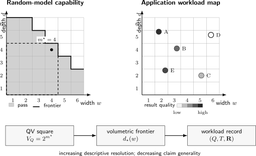
One scalar, one capability map, and many workloads. The quantum-volume point is the largest certified square under a random-circuit frontier. A volumetric map retains rectangular width–depth tradeoffs. Application circuits then occupy particular regions and carry their own quality, time, and resource coordinates; equal circuit shape does not guarantee equal workload behavior.

The circuit family remains part of the benchmark. A pass map for random two-qubit layers need not transfer to Fourier circuits, Hamiltonian simulation, mid-circuit measurement, dynamic feed-forward, or error-correction cycles.

From Generic Circuits to Application-Oriented Tests

An algorithm name is not yet a benchmark. “Run QFT,” “run VQE,” or “run QAOA” leaves open the input, circuit construction, accuracy target, optimizer, measurement budget, and reference answer. An application-oriented benchmark must convert a scientific intention into an executable contract.

A useful abstract specification is

$$\mathcal B = \left( \mathcal T, \Pi, \mathcal I, \mathcal R, \mathcal Q, \mathcal C, \mathcal A \right),$$

where:

• $\mathcal T$ is the task and problem-size parameter;
• $\Pi$ is the input or instance distribution;
• $\mathcal I$ is the implementation policy;
• $\mathcal R$ is the reference-answer procedure;
• $\mathcal Q$ is the result-quality metric;
• $\mathcal C$ is the resource and timing contract;
• $\mathcal A$ is the statistical acceptance rule.

Changing any component can change the measured capability. Benchmark names and scalar scores should never replace the full tuple.

Application, application-oriented, and algorithmic

These terms should be used carefully:

• An application benchmark represents an end-to-end task of genuine intended use, with an operationally meaningful output criterion.
• An application-oriented benchmark uses a circuit or subroutine motivated by an application, but may simplify the input, oracle, optimizer, or output.
• An algorithmic benchmark tests a specified algorithm or primitive and need not establish practical utility.

A Fourier transform followed by an easily predicted inverse can test coherent control without being a useful standalone application. A tiny chemistry instance can test an end-to-end workflow while remaining classically trivial. Precise labels prevent “application-inspired” from being inflated into “practically useful.”

Designing the Instance Ensemble

Results can vary more across instances than across devices. A mature benchmark therefore defines:

1. the population of admissible instances;
2. the sampling distribution or fixed public corpus;
3. stratification by size, density, symmetry, condition number, or other difficulty variables;
4. training, development, and held-out test partitions;
5. random seeds and duplicate handling;
6. rules for failed, timed-out, or infeasible instances.

The target quantity is usually an expectation or quantile over the declared instance distribution:

$$\mu_Q(n) = \mathbb E_{I\sim\Pi_n} \left[ Q(I) \right].$$

Reporting only the easiest instance estimates a different quantity. So does allowing each platform to choose a different subset. If instance selection must differ because of device constraints, the comparison should either restrict all systems to the common subset or present the results as non-equivalent case studies.

Held-out instances matter whenever compilation, ansatz selection, mitigation, hyperparameters, or calibration decisions can adapt to observed scores. Without a separation between tuning and evaluation, benchmark optimization can overfit the public suite.

Quality Metrics

The score should reflect the task’s output, not merely circuit survival. Common choices include:

task output	possible quality quantity
one correct bit string	success probability
sampled distribution	total variation, Hellinger distance, fidelity, or task statistic
observable estimate	absolute or normalized estimation error
ground-state energy	energy error relative to a trusted reference
optimization candidate	feasible objective value or approximation ratio
simulation trajectory	error over a declared set of observables and times
encoded operation	logical failure probability per declared opportunity

No quality metric is universally appropriate. Distribution fidelity can hide a wrong rare event that dominates a risk-sensitive task. Mean energy can look accurate for a poor state. Approximation ratios require carefully chosen sign conventions and baselines. Observable error says nothing about unmeasured observables.

Where possible, report both the task metric and one diagnostic quantity. The task metric establishes usefulness under the contract; the diagnostic helps explain failure.

A Normalized Distribution Score

One application-oriented suite uses the squared Bhattacharyya coefficient, often called classical fidelity:

$$F_{\mathrm s}(p,q) = \left( \sum_x\sqrt{p_xq_x} \right)^2.$$

It satisfies $0\leq F_{\mathrm s}\leq 1$ and equals one when $p=q$. To set a uniform-output baseline $u_x=1/D$ to zero, define

$$F_{\mathrm{raw}}(p,q) = \frac{ F_{\mathrm s}(p,q)-F_{\mathrm s}(p,u) }{ 1-F_{\mathrm s}(p,u) }.$$

The suite convention then clips negative values:

$$F(p,q) = \max \left\{ F_{\mathrm{raw}}(p,q),0 \right\}.$$

This normalization is convenient across circuits whose ideal distributions have different concentration. It is not a universal fidelity theorem. Clipping makes the plotted scale nonnegative but hides whether a result is slightly or strongly worse than the uniform baseline. For diagnostic work, retain and publish $F_{\mathrm{raw}}$ as well. If $p=u$, the denominator vanishes; that target needs a different score or a benchmark construction whose ideal output is not uniform.

Finite-shot plug-in estimates of nonlinear quantities such as $F_{\mathrm s}$ can be biased. The uncertainty method should reproduce the whole estimator, including finite-shot histograms, mitigation, normalization, and averaging across instances.

Accuracy Before Speed

A fast wrong answer is not a successful benchmark. Performance should be reported at a declared accuracy:

$$T(\epsilon,n), \qquad R(\epsilon,n),$$

where $T$ is elapsed time, $R$ is a resource vector, $n$ is problem size, and $\epsilon$ defines the accepted output error. If the natural criterion is a success probability, write

$$p_{\mathrm{succ}}(n)\geq p_\star.$$

Cross-platform speed comparisons should use the same task and quality target, or provide a quality–time frontier. Comparing one platform at low accuracy with another at high accuracy answers no stable performance question.

Time to solution

A useful end-to-end timing decomposition is

$$\begin{aligned} T_{\mathrm{total}} &= t_{\mathrm{compile}} +t_{\mathrm{queue}} +t_{\mathrm{setup}} \\ &\quad+ \sum_{r=1}^{R} \left( t_{\mathrm{classical},r} +t_{\mathrm{submit},r} +t_{\mathrm{QPU},r} +t_{\mathrm{readout},r} \right) \\ &\quad+ t_{\mathrm{post}} +t_{\mathrm{verify}}. \end{aligned}$$

Different questions include different terms:

• QPU execution time isolates scheduled quantum work.
• dedicated-system latency may exclude public-cloud queueing.
• user-observed wall time includes queueing and API overhead.
• amortized throughput may spread compilation and setup across a batch.
• time to solution includes all repeated attempts needed to satisfy the output criterion.

Report the boundary rather than using “runtime” without definition. Provider API timing fields are not automatically comparable; their start and stop events must be documented.

For an independent run with success probability $p_{\mathrm{succ}}$, the number of repetitions required for cumulative confidence at least $\gamma$ is

$$R_\gamma = \left\lceil \frac{\ln(1-\gamma)} {\ln(1-p_{\mathrm{succ}})} \right\rceil.$$

If each run takes $t_{\mathrm{run}}$, then

$$\operatorname{TTS}_\gamma = R_\gamma t_{\mathrm{run}}.$$

This formula assumes independent, stationary repetitions. Drift, shared calibration failures, adaptive restarts, and correlated decoding errors can invalidate it.

Resource Accounting

Time alone can hide expensive substitution between resources. Record a vector such as

$$\mathbf R = \left( n_{\mathrm{phys}}, n_{\mathrm{log}}, N_{1q}, N_{2q}, D_{\mathrm{native}}, N_{\mathrm{shots}}, C_{\mathrm{class}}, M_{\mathrm{class}} \right),$$

where the entries may denote physical and logical qubits, native gate counts, native scheduled depth, shots, classical operations, and classical memory. Add communication, cryogenic duty cycle, decoder work, energy, monetary cost, or failed attempts when they are material to the claim.

For fault-tolerant workloads, logical circuit counts without code distance, factory assumptions, decoder latency, and physical-error model are insufficient. Resource Estimation Tools develops that accounting in detail.

Circuit depth is especially policy dependent. Three commonly confused quantities are:

• depth in the high-level algorithmic representation;
• depth after lowering to a standardized hardware-agnostic basis;
• scheduled depth or duration in native operations.

Application-suite plots may use a standardized depth to compare circuit footprints, but hardware execution claims should also report the actual native schedule.

Building a Representative Suite

One workload cannot represent a computational platform. A suite should span features that stress different parts of the stack:

• sparse and dense logical connectivity;
• serial and highly parallel operations;
• shallow and deep circuits;
• different fractions of entangling gates;
• mid-circuit measurement, reset, and feed-forward;
• parameter updates and hybrid quantum–classical loops;
• sampling, expectation estimation, and decision outputs;
• noise-sensitive and symmetry-protected structures.

Feature vectors can diagnose suite coverage, but geometric coverage in a chosen feature space does not prove coverage of all applications. The feature map itself is a modeling choice, and two circuits with similar gate counts can respond differently to coherent or correlated errors.

Suites should evolve. A fixed suite eventually invites specialized compiler paths, memorized instances, and hardware tuned to the public tests. Versioned releases, hidden or rotating instances, deprecation rules, and historical re-runs are part of long-lived benchmark governance.

Important Benchmark Families

Several established proposals illustrate complementary design choices:

• Quantum volume uses synthetic random model circuits and a binary heavy-output threshold to obtain a compact full-stack score.
• Volumetric benchmarks retain a width–depth capability map and allow the circuit ensemble and success criterion to vary.
• Application-motivated full-stack tests use deep, shallow, and square circuit classes to expose interactions between workload, compiler, and hardware.
• QED-C application-oriented benchmarks sweep problem size across tutorial, subroutine, and functional circuit families and report result quality, timing, and gate resources.
• SupermarQ emphasizes scalable application-level circuits, explicit workload features, suite coverage, and cross-architecture execution.
• throughput complements, such as the proposed circuit-layer-operations metric, target speed dimensions that quantum volume omits.

These are examples, not interchangeable standards. Their source circuits, score conventions, compiler freedoms, timing boundaries, and suite versions must accompany any numerical comparison.

Suite Aggregation and Pareto Frontiers

Suppose a suite produces normalized scores $s_1,\ldots,s_J$. A weighted geometric mean,

$$S_{\mathrm{geo}} = \prod_{j=1}^{J}s_j^{w_j}, \qquad \sum_j w_j=1,$$

can be useful only when every score is positive, similarly oriented, and meaningfully normalized. The weights encode a workload distribution, not a law of nature. Different weights can reverse a ranking.

A single aggregate also hides catastrophic failure on one task. At minimum, publish:

• every task score and uncertainty;
• median and lower-tail performance across instances;
• timing and resources at matched accuracy;
• the aggregation formula and weights;
• missing, timed-out, and unsupported cases.

Often the honest result is a Pareto set. System $A$ may dominate in latency while $B$ uses fewer shots, or $A$ may excel on shallow dense circuits while $B$ sustains deeper sparse ones. A scalar ranking requires an external utility function.

Statistical Design for Application Suites

Application results usually have more levels than a Bernoulli shot model:

$$\text{day} \supset \text{calibration} \supset \text{instance} \supset \text{mapping} \supset \text{shot}.$$

Uncertainty should match the target population:

• Resample shots to quantify measurement noise for one fixed circuit.
• Resample instances to generalize to the declared problem distribution.
• Resample mappings when placement is random under the contract.
• Repeat across time blocks to quantify drift and service variability.
• Repeat optimization seeds for stochastic hybrid algorithms.

If the claim concerns future user workloads, an interval conditional on one hand-picked instance and one favorable calibration is too narrow. Report between-instance and between-time variation rather than pooling every shot.

Multiple task sizes and score thresholds also create multiplicity. A benchmark that searches many shapes and publishes only the best passing point needs a selection-aware confidence rule or held-out confirmation. The same logic applies to searching qubit subsets, compiler seeds, ansatzes, and mitigation hyperparameters.

Fair Cross-Platform Comparisons

A comparison is interpretable only after fixing the comparison object.

Same source task

Use the same problem definition, instance distribution, output criterion, and problem sizes. Platform-specific source implementations may be necessary, but they should implement the same mathematical task.

Same policy, not necessarily identical gates

Different architectures need different native gates. Fairness usually means equal freedom and resource accounting, not forcing both platforms into an unnatural common instruction set. Declare whether each stack may:

• optimize freely;
• select qubits or zones;
• use approximate synthesis;
• apply mitigation or postselection;
• batch circuits;
• cache compilation;
• exploit dynamic circuits or analog primitives.

Same tuning budget

Count human and machine tuning effort when it affects the result. A hand-optimized implementation developed for weeks should not be compared with an untouched default compiler without saying so.

Same accuracy and failure treatment

Match output accuracy, confidence, timeout, and retry rules. Include failed runs in the denominator unless the protocol predeclares a scientifically justified rejection rule.

Classical baselines

Use a strong, current classical method on appropriate hardware, with matched accuracy and complete resource accounting. A quantum system beating a weak baseline does not establish advantage. Conversely, an application benchmark can be useful for diagnosing quantum systems even when every tested instance is easy classically.

A Defensible Workflow

1. State the question. Decide whether the target is hardware diagnosis, delivered-stack capability, application quality, throughput, or advantage.
2. Freeze the contract. Version the task, instances, circuit generators, compiler freedom, score, timing boundary, resources, and acceptance rule.
3. Validate references. Check ideal answers on analytically solvable cases and overlapping independent simulators.
4. Separate tuning and test data. Freeze all adaptive choices before held-out evaluation.
5. Collect hierarchical data. Sample enough circuits or instances, not merely many shots of one object; repeat across relevant time blocks.
6. Preserve artifacts. Store source and native circuits, seeds, mappings, calibration records, counts, timings, failures, and software environments.
7. Analyze the declared estimand. Use uncertainty and multiplicity corrections appropriate to the sampling hierarchy.
8. Publish the surface. Show per-size quality, time, and resources before any aggregate score.
9. Stress-test conclusions. Vary compiler policy, instance strata, and reasonable classical baselines.
10. Scope the claim. Say exactly which system version, workload distribution, accuracy, and date the evidence supports.

Reproducible Notebooks provides a practical artifact structure for this workflow.

Minimum Reporting Record

Quantum volume

• protocol and software version;
• random-circuit seeds and number of circuits per shape;
• shots per circuit and time-block structure;
• ideal-simulation method and numerical precision;
• compiler, approximation, mapping, and subset-selection policy;
• native gate counts, scheduled depth, and chosen physical qubits;
• raw per-circuit heavy fractions;
• confidence method, level, and pass/fail rule;
• calibration timestamp and all mitigation or postselection;
• every tested shape, not only the largest pass.

Application-oriented suite

• suite and circuit-generator version;
• task definition, instance distribution, and tested sizes;
• held-out policy and tuning budget;
• reference-answer method and its uncertainty;
• quality metric, normalization, and acceptance target;
• compiler and native execution artifacts;
• timing start and stop events;
• quantum, classical, and service resources;
• failed, rejected, and timed-out runs;
• hierarchical uncertainty and aggregation rule;
• hardware, firmware, software, calibration, and collection dates.

Common Mistakes

Treating quantum volume as usable qubit count

$V_Q=2^m$ does not mean the processor has $2^m$ qubits. The exponent $m$ is a certified random-circuit width–depth scale.

Passing on the point estimate

$\widehat h>2/3$ is not the protocol’s statistical claim. The one-sided lower confidence bound must exceed $2/3$ under the declared independent units.

Replacing circuits by shots

One million shots of ten circuits do not provide the same evidence about the random-circuit ensemble as many independent circuits.

Hiding the compiler and selected subset

Quantum volume is full-stack. Compiler and placement improvements are valid, but undisclosed search changes the estimand and invalidates naive uncertainty.

Extrapolating the square everywhere

The largest passing square does not determine wide-shallow, narrow-deep, dynamic-circuit, or application performance. Measure the relevant region and circuit family.

Calling every proxy an application

A tutorial oracle or efficiently checkable subroutine may be an excellent system test without demonstrating practical utility.

Comparing runtime at unequal quality

Speed is meaningful only with a task, an accuracy target, and declared failure handling.

Averaging away failures

An attractive suite mean can coexist with a failed workload class or a severe lower tail. Publish the distribution and unsupported cases.

Proving advantage with a benchmark score

System quality is only one ingredient. Advantage needs a strong classical baseline, resource comparison, verification argument, and claim-specific analysis.

Research Status

The quantum-volume protocol, heavy-output test, and volumetric generalization are established benchmarking methods. Application-oriented suites are also an established and actively developed approach to full-stack evaluation.

Important choices remain active rather than standardized: representative workload sets, circuit-depth normalization, timing boundaries, mitigation rules, hidden-instance governance, logical-workload metrics, cross-platform compiler fairness, and scalable verification beyond exact classical simulation. Benchmark suites should therefore be cited by version and date.

The durable conclusion is modest but useful: no scalar predicts all quantum workloads. Trustworthy evidence is a layered record of quality, speed, resources, uncertainty, and scope.

Further Connections

• Why Benchmarking Is Hard develops the general benchmark contract, selection effects, verification ladder, and evidence hierarchy.
• Algorithmic Benchmarking carries an application-shaped circuit suite into a complete named-algorithm benchmark with input, hybrid-loop, acceptance, retry, and scaling costs.
• Cross-Entropy Benchmarking treats a different random-circuit score and its conditional fidelity interpretation.
• Randomized Benchmarking estimates sequence-decay parameters rather than workload-level success.
• Cycle Benchmarking probes fixed scheduled layers using Pauli randomization.
• Metrics for Quantum Hardware compares component, gate, system, logical, and service estimands.
• Quantum Software Stack identifies the layers included in a full-stack score.
• Error-Aware Compilation explains calibration-sensitive placement and held-out compiler evaluation.
• Calibration Loops develops drift monitoring and acceptance gates.
• Quantum Circuit Simulation supplies exact and approximate reference calculations.
• Resource Estimation Tools develops physical, logical, classical, and uncertainty-aware resource estimates.
• Claims, Hype, and Evidence Standards separates measured capability from utility and advantage claims.
• Validation Tests supplies checks for benchmark implementations and computational artifacts.

References

1. A. W. Cross, L. S. Bishop, S. Sheldon, P. D. Nation, and J. M. Gambetta, “Validating quantum computers using randomized model circuits,” Physical Review A 100, 032328 (2019), doi:10.1103/PhysRevA.100.032328.
2. S. Aaronson and L. Chen, “Complexity-theoretic foundations of quantum supremacy experiments,” Proceedings of the 32nd Computational Complexity Conference, 22:1–22:67 (2017), doi:10.4230/LIPIcs.CCC.2017.22.
3. R. Blume-Kohout and K. C. Young, “A volumetric framework for quantum computer benchmarks,” Quantum 4, 362 (2020), doi:10.22331/q-2020-11-15-362.
4. T. Proctor, K. Rudinger, K. Young, E. Nielsen, and R. Blume-Kohout, “Measuring the capabilities of quantum computers,” Nature Physics 18, 75–79 (2022), doi:10.1038/s41567-021-01409-7.
5. D. Mills, S. Sivarajah, T. L. Scholten, and R. Duncan, “Application-motivated, holistic benchmarking of a full quantum computing stack,” Quantum 5, 415 (2021), doi:10.22331/q-2021-03-22-415.
6. T. Lubinski et al., “Application-oriented performance benchmarks for quantum computing,” IEEE Transactions on Quantum Engineering 4, 3100316 (2023), doi:10.1109/TQE.2023.3253761.
7. T. Tomesh et al., “SupermarQ: A scalable quantum benchmark suite,” 2022 IEEE International Symposium on High-Performance Computer Architecture, 587–603 (2022), doi:10.1109/HPCA53966.2022.00050.
8. A. Wack et al., “Quality, speed, and scale: three key attributes to measure the performance of near-term quantum computers,” arXiv:2110.14108 (2021), arXiv:2110.14108. This is a white paper and preprint; metric definitions and implementations can evolve.
9. J. Dongarra, P. Luszczek, and A. Petitet, “The LINPACK benchmark: past, present and future,” Concurrency and Computation: Practice and Experience 15, 803–820 (2003), doi:10.1002/cpe.728.
10. J. L. Hennessy and D. A. Patterson, Computer Architecture: A Quantitative Approach, 6th ed., Morgan Kaufmann (2019), chapters 1 and 2.
11. A. Elben et al., “The randomized measurement toolbox,” Nature Reviews Physics 5, 9–24 (2023), doi:10.1038/s42254-022-00535-2.
12. M. Kliesch and I. Roth, “Theory of quantum system certification,” PRX Quantum 2, 010201 (2021), doi:10.1103/PRXQuantum.2.010201.

Exercises

1. Derive the ideal heavy-output probability

Assume $z=Dp$ has density $e^{-z}$ for $z\geq0$. Derive the median threshold and the ideal heavy-output probability. Explain why the latter is not $1/2$.

Solution

The median obeys

$$1-e^{-z_{\mathrm{med}}} = \frac{1}{2},$$

so $z_{\mathrm{med}}=\ln2$. Half the labels lie above this value. An ideal sample selects labels with probability proportional to $p$, producing the size-biased density $z e^{-z}$. Therefore

$$\begin{aligned} h_{\mathrm{ideal}} &= \int_{\ln2}^{\infty}z e^{-z}\,dz \\ &= \frac{1+\ln2}{2} \approx0.8466. \end{aligned}$$

The distinction is between uniformly sampling labels and sampling from the ideal quantum distribution.

2. Convert the threshold under a noise model

For $q_F=Fp+(1-F)u$, derive the asymptotic heavy-output probability and the minimum $F$ needed to exceed $2/3$. State one reason not to call this $F$ a measured process fidelity in general.

Solution

Linearity gives

$$\begin{aligned} h_F &= F\frac{1+\ln2}{2} + (1-F)\frac12 \\ &= \frac12+\frac{F\ln2}{2}. \end{aligned}$$

Demanding $h_F>2/3$ yields

$$F>\frac{1}{3\ln2}\approx0.4809.$$

The conversion assumes one global depolarizing mixture. Coherent, circuit-dependent, leakage, correlated, or readout errors can give the same heavy-output score without satisfying that model, so $F$ is not a general process-fidelity estimate.

3. Separate shots from circuits

A team tests $K=20$ circuits with $S=10\,000$ shots each and reports a Bernoulli standard error based on $KS=200\,000$ independent trials. What variation is omitted, and how should the experiment be improved?

Solution

The analysis omits the between-circuit term

$$\frac{\operatorname{Var}_U(h_U)}{K}.$$

Shots within one circuit estimate that circuit’s $h_U$; they do not create new draws from the circuit ensemble. The team should sample at least the required number of independent circuits, retain per-circuit estimates, and use a circuit-level interval or hierarchical bootstrap. Once shot noise is small, adding circuits is much more valuable than adding shots.

4. Compute a quantum volume

Suppose

$$d_\star(2)=9,\quad d_\star(3)=7,\quad d_\star(4)=4,\quad d_\star(5)=3.$$

Compute $V_Q$. Which capability information is discarded by the scalar?

Solution

The values of $\min\{m,d_\star(m)\}$ are $2,3,4,3$. Hence

$$\log_2V_Q=4, \qquad V_Q=16.$$

The scalar discards the fact that widths two and three sustain depths far beyond four, the pass margins at each shape, uncertainty, failure behavior at larger shapes, and all dependence on circuit families other than the random model ensemble.

5. Diagnose a compiler comparison

System $A$ may search 500 qubit mappings and use approximate synthesis. System $B$ uses one fixed mapping and exact synthesis. $A$ has larger quantum volume. Give two valid interpretations and one invalid interpretation.

Solution

A valid interpretation is that the delivered stack $A$, with its declared search and approximation policy, performs better on this protocol. Another is that compilation freedom materially affects the score and deserves separate study. It is invalid to conclude that $A$‘s hardware gates are intrinsically better, because hardware, mapping search, and synthesis policy were not controlled. A hardware-focused comparison would equalize policy as far as the architectures permit and report native schedules and approximation error.

6. Examine normalized result fidelity

Let the ideal distribution be $p=(3/4,1/4)$, the measured distribution be $q=(1/2,1/2)$, and $u=(1/2,1/2)$. Compute $F_{\mathrm s}(p,q)$ and $F_{\mathrm{raw}}(p,q)$.

Solution

Because $q=u$,

$$F_{\mathrm s}(p,q) = \left( \sqrt{\frac{3}{8}} + \sqrt{\frac{1}{8}} \right)^2 = \frac{2+\sqrt3}{4}.$$

The same value appears in the baseline term $F_{\mathrm s}(p,u)$. Therefore

$$F_{\mathrm{raw}}(p,q)=0.$$

The normalization says that the measured result is no better than uniform for this ideal target, even though the unnormalized classical fidelity is close to one.

7. Compute time to solution

One run takes $0.40$ s and succeeds independently with probability $0.20$. How many runs are needed for at least $99\%$ cumulative success, and what is the resulting time to solution?

Solution

Use

$$R_{0.99} = \left\lceil \frac{\ln(0.01)}{\ln(0.8)} \right\rceil = 21.$$

Thus

$$\operatorname{TTS}_{0.99} = 21(0.40\ \mathrm{s}) = 8.4\ \mathrm{s}.$$

The result assumes stationary independent runs and excludes any setup, queueing, or verification costs not included in the stated $0.40$ s.

8. Design a fair application benchmark

Two providers are to be compared on a variational ground-state task. List a minimum contract that prevents the most obvious accuracy, tuning, and timing ambiguities.

Solution

Fix the Hamiltonian family and held-out instance distribution; problem sizes; target energy error and confidence; ansatz freedoms; optimizer and stopping rules or equal tuning budget; initialization and random seeds; shot and mitigation policy; compiler and placement freedom; treatment of failed runs; reference-energy method; and the timing boundary. Record source and native circuits, every quantum and classical iteration, calibration state, raw measurements, wall time, QPU time, and classical resources. Report quality– time–resource curves per size before any suite aggregate.