Calibration Loops

Short Definition

A calibration loop is a versioned supervisory process that keeps a quantum device within a declared operating region. It observes health indicators or scheduled triggers, chooses calibration experiments, estimates parameters, proposes a candidate control snapshot, validates that candidate on data not used to fit it, and then either publishes, rejects, rolls back, or quarantines the affected resources.

The loop is not just a numerical optimizer. A production-quality loop must answer:

• which parameter or operation is being calibrated;
• which upstream records and physical context the result depends on;
• what data, likelihood, estimator, and uncertainty statement produced it;
• which resources the experiment occupies or perturbs;
• which descendants become stale when the value changes;
• what held-out evidence is required before publication;
• how the update is made atomic for queued and running programs;
• when the result expires or becomes suspect;
• which previous snapshot can be restored, and what must be revalidated after restoration.

This page owns that orchestration contract. Control, Readout, and Calibration owns the physical delivery and observation chain, the basic calibration estimands, and representative tune-up experiments. Rabi and Ramsey Control owns the canonical driven two-level derivations. Pulse-Level Control owns the executable waveform, frame, sample-grid, and pulse-certificate contract. Calibration loops decide when and how those artifacts are estimated, qualified, versioned, and replaced.

A Versioned Supervisory Control System

Let $S_n$ be the active calibration snapshot before maintenance cycle $n$. A minimal loop can be represented as

$$\begin{aligned} S_n &\xrightarrow{\ \Pi\ } X_n \xrightarrow{\ \mathrm{device}\ } D_n \xrightarrow{\ \mathcal A\ } \widetilde S_{n+1} \\ &\xrightarrow{\ \mathcal Q\ } \left\{ \begin{array}{ll} S_{n+1}, & \text{publish},\\ S_n, & \text{retain or roll back},\\ \bot, & \text{quarantine}. \end{array} \right. \end{aligned}$$

Here:

• $S_n$ contains immutable parameter records and their dependency versions;
• $\Pi$ is a planner that selects experiments and an execution order;
• $X_n$ is the resulting batch of circuits, pulses, settings, and resource reservations;
• $D_n$ is the timestamped measurement and telemetry record;
• $\mathcal A$ is the analysis and estimation procedure;
• $\widetilde S_{n+1}$ is a candidate snapshot;
• $\mathcal Q$ is a qualification policy with statistical and engineering acceptance criteria;
• $\bot$ means that no trusted operating snapshot is available for the affected scope.

The third outcome matters. If both the candidate and incumbent fail safety or validity checks, silently keeping the incumbent is not conservative. The correct action may be to stop admitting workloads to a qubit, coupler, mode, readout group, or full processor partition.

Calibration is usually feedback between experiments, not feedback within one quantum trajectory. A measurement-based quantum controller may need to act within microseconds or less. A calibration controller may aggregate thousands of shots and update the next batch seconds or hours later. Some modern controllers blur this distinction, but the latency, state estimate, and safety contract should still identify which loop is being discussed.

The Calibration Record

A scalar value without context is not a calibration. For a node $v$, a useful record is

$$\begin{aligned} r_v = \bigl( &\widehat\theta_v,\, \Sigma_v,\, \mathcal D_v,\, \mathcal M_v,\, \mathcal P_v,\, \mathcal C_v, \\ &t_v,\, I_v,\, q_v,\, h_v,\, \rho_v \bigr). \end{aligned}$$

The fields denote, respectively:

• the estimate $\widehat\theta_v$ and uncertainty $\Sigma_v$;
• the data reference $\mathcal D_v$ and analysis/model version $\mathcal M_v$;
• parent record hashes $\mathcal P_v$;
• the operating-context domain $\mathcal C_v$;
• acquisition time $t_v$ and validity interval $I_v$;
• qualification evidence $q_v$;
• health indicators $h_v$;
• provenance and rollback metadata $\rho_v$.

The estimate can be a scalar frequency, a waveform parameter vector, a confusion matrix, a transfer function, or an entire model. The uncertainty may be a covariance matrix, posterior samples, a confidence region, or a protocol-specific interval. Whatever representation is used, it must retain the assumptions needed to interpret it.

A validity predicate

At execution time $t$ and context $c$, a record should be consumed only if a machine-checkable predicate holds. One schematic form is

$$\begin{aligned} \operatorname{Valid}_v(t,c;S) \equiv{}& \mathbf 1[t\in I_v]\, \mathbf 1[c\in\mathcal C_v] \\ &\land \mathbf 1[\mathcal P_v=\operatorname{head}_S(\operatorname{Pa}(v))] \\ &\land \mathbf 1[h_v(t)\in\mathcal H_v]\, \mathbf 1[q_v\ \mathrm{passes}]. \end{aligned}$$

This separates several operational states:

• valid: every declared condition passes;
• suspect: monitoring has raised evidence of change, but invalidity has not yet been established;
• stale: a parent version, time limit, or context condition no longer matches;
• invalid: a required acceptance or safety condition has failed;
• unknown: required evidence is absent or the monitor itself is unhealthy.

Unknown is not equivalent to valid, and stale is not a synonym for physically bad. A stale pulse may still work; the point is that its previous claim no longer covers the current context.

Dependencies and Invalidation

Calibration procedures are often bootstrapped. A readout classifier may depend on resonator frequency and amplifier state. A drive-amplitude calibration may depend on drive frequency, duration, transfer correction, and the classifier used to interpret outcomes. An entangling operation may depend on both single-qubit frames, coupler bias, neighbor state, and simultaneous-drive context.

Represent these dependencies by a directed graph

$$G_{\mathrm{cal}}=(V,E), \qquad u\longrightarrow v \quad\Longleftrightarrow\quad r_v\ \text{was qualified using}\ r_u.$$

If a set $A\subseteq V$ changes, the conservative invalidation set is

$$\operatorname{Inv}(A) = A\cup\operatorname{Desc}_{G_{\mathrm{cal}}}(A).$$

Blindly invalidating every descendant can be prohibitively expensive. A more precise edge carries an impact contract: which parent fields matter, what change magnitude is material, and which contexts are affected. If a readout frequency shifts within a tolerance already covered by a classifier’s robust validation region, the classifier need not automatically be refit. That decision must follow recorded evidence, not operator intuition.

Cycles mean the node boundary is wrong

A true directed acyclic graph admits a topological execution order. Real calibration dependencies can appear cyclic: drive amplitude affects measured detuning, while the detuning estimate affects the amplitude fit. Treating that as an impossible graph is unhelpful. Instead, either:

1. group the coupled parameters into one calibration node;
2. define a fixed-point iteration with a convergence and stopping policy; or
3. break the cycle with a declared approximation and validate its residual.

The software dependency graph is also not the hardware resource graph. Two nodes can be logically independent yet unable to run concurrently because they share a readout line, laser, microwave source, cryogenic budget, or disturb one another through crosstalk.

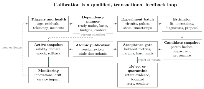
Routine calibration is a transactional feedback process. A dependency-aware planner turns health evidence into experiments; a candidate becomes active only after held-out acceptance and an atomic commit. Rejection preserves the incumbent when it remains valid, while unsafe or ambiguous cases are quarantined. Monitoring closes the slower supervisory loop.

Operating Regimes

Calibration is not one workflow at one cadence.

Regime	Starting information	Main task	Typical completion criterion
commissioning	little or no trusted state	discover operating regions and bootstrap dependencies	a complete qualified base snapshot
tune-up	approximately correct parameters	reduce a known objective locally	candidate beats or is noninferior to incumbent
maintenance	an active snapshot plus monitors	detect staleness and refresh selected nodes	validity restored with bounded interruption
incident recovery	failed health or validation checks	localize failure and find a safe state	affected scope recovered or quarantined
in-situ tracking	low-latency diagnostic stream	follow a drifting latent parameter	tracking error remains within a declared bound

Commissioning may require wide scans and conservative hardware limits. Maintenance should usually start from the incumbent, use smaller experiment budgets, and avoid perturbing unrelated controls. Incident recovery should preserve evidence from the failure rather than overwriting it with a fresh successful fit.

An in-situ loop must be distinguished from error correction. A decoder infers discrete errors or a logical state from syndrome records under a code model. A calibration tracker estimates slowly or intermittently varying control parameters. Syndrome data can inform calibration, but using it for both tasks creates coupled estimators whose assumptions and latencies must be stated.

Drift as Latent-State Estimation

Repeated recalibration from scratch discards useful temporal structure. A simple state-space model is

$$\begin{aligned} \theta_{k+1} &= F_k\theta_k+w_k, & w_k&\sim(0,Q_k), \\ y_k &= h_k(\theta_k,x_k)+v_k, & v_k&\sim(0,R_k), \end{aligned}$$

where $\theta_k$ is the latent device or control state, $x_k$ is the chosen experiment, and $y_k$ is the observation. The process covariance $Q_k$ expresses expected motion; the measurement covariance $R_k$ expresses observation noise. These are modeling statements, not properties supplied by the device.

For a linear model, a Kalman-style update is

$$\begin{aligned} \widehat\theta_{k|k-1} &= F_{k-1}\widehat\theta_{k-1|k-1}, \\ P_{k|k-1} &= F_{k-1}P_{k-1|k-1}F_{k-1}^{\mathsf T} +Q_{k-1}, \\ K_k &= P_{k|k-1}H_k^{\mathsf T} \left( H_kP_{k|k-1}H_k^{\mathsf T}+R_k \right)^{-1}, \\ \widehat\theta_{k|k} &= \widehat\theta_{k|k-1} +K_k \left( y_k-H_k\widehat\theta_{k|k-1} \right), \\ P_{k|k} &= (I-K_kH_k)P_{k|k-1}. \end{aligned}$$

This form is useful for slowly varying frequencies, phases, gains, positions, or crosstalk coefficients when the local model is credible. Nonlinear, multimodal, constrained, or abruptly switching systems may require extended filters, particle methods, hidden-state models, or explicit change-point detection.

The estimated covariance is only in-model uncertainty. A small $P_{k|k}$ does not protect against a wrong transfer model, an unmodeled level, misclassified readout, a changed wiring state, or a regime switch. Residual checks and independent validation remain necessary.

Monitoring Without Chasing Noise

A monitor should detect operationally meaningful change without turning every statistical fluctuation into a parameter update. If a health measurement has prediction $\widehat y_k$ and innovation variance $S_k$, define the standardized innovation

$$z_k = \frac{y_k-\widehat y_k}{\sqrt{S_k}}.$$

A single threshold on $|z_k|$ catches abrupt excursions but is insensitive to small persistent shifts. A two-sided cumulative-sum monitor can use

$$\begin{aligned} C_k^+ &= \max\!\left(0,C_{k-1}^++z_k-\kappa\right), \\ C_k^- &= \max\!\left(0,C_{k-1}^--z_k-\kappa\right), \end{aligned}$$

and trigger when either statistic exceeds $h$. The allowance $\kappa$ sets the shift scale of interest; $h$ trades detection delay against false alarms. Correlated data, estimated baselines, and repeated monitoring alter the nominal false-alarm rate, so thresholds should be calibrated under the actual acquisition protocol.

Cadence, event triggers, and hysteresis

Useful trigger classes include:

• fixed cadence for slow, predictable aging;
• age or validity-interval expiration;
• thresholded health telemetry;
• residual or change-point evidence;
• upstream parameter publication;
• workload-specific preflight checks;
• operator or incident-response requests.

A warning threshold and a stricter stop threshold prevent a marginal signal from immediately removing a resource from service. A reset threshold lower than the trigger threshold provides hysteresis. Minimum dwell times and cooldowns can prevent rapid toggling, but they must not suppress a genuine safety event.

Monitoring many qubits, edges, and metrics creates a multiple-testing problem. Reporting the most extreme trace from thousands of monitors without correcting for selection will manufacture apparent anomalies. False-discovery control, hierarchical alarms, spatial correlation models, or confirmatory tests can reduce alarm floods.

Which Calibration Runs Next?

The oldest record is not necessarily the most urgent. A useful risk quantity is

$$\mathcal R_v(t) = \Pr\!\left( \neg\operatorname{Valid}_v(t,c) \mid\mathcal D_{\le t} \right) L_v,$$

where $L_v$ is the expected operational loss if node $v$ is invalid. A heuristic priority score might be

$$\pi_v = \frac{\mathcal R_v} {N_v+\lambda T_v+\mu B_v},$$

where $N_v$ is shot cost, $T_v$ is wall-clock cost, and $B_v$ measures disturbance or blocked workload. This is not a universal objective. The weights and loss must be tied to the service being protected.

The scheduler must also enforce:

• calibration dependencies and invalidation consequences;
• exclusive and shared hardware resources;
• concurrency contexts that have been qualified;
• warm-up, cooldown, reset, and settling times;
• experiment deadlines and snapshot expirations;
• fair access between calibration and user workloads;
• a maximum scope for simultaneous changes.

Independent graph nodes may run in parallel only when their physical resource sets and disturbance domains are compatible. Conversely, jointly calibrated controls may need to run as one node even when their software records are stored separately.

Update Dynamics and Loop Stability

Calibration software can destabilize an otherwise usable device by applying updates too aggressively. Consider a fixed true parameter $\theta^\star$, an estimate $\widehat\theta_n$, and a noisy signed error observation

$$y_n = \theta^\star-\widehat\theta_n+\varepsilon_n, \qquad \mathbb E[\varepsilon_n]=0, \qquad \operatorname{Var}(\varepsilon_n)=\sigma^2.$$

For the proportional update

$$\widehat\theta_{n+1} = \widehat\theta_n+g\,y_n,$$

the estimation error $e_n=\theta^\star-\widehat\theta_n$ obeys

$$e_{n+1} = (1-g)e_n-g\varepsilon_n.$$

The noiseless loop is asymptotically stable exactly when

$$|1-g|<1, \qquad\text{or}\qquad 0<g<2.$$

For independent measurement noise and a stationary true parameter, the steady-state error variance is

$$\operatorname{Var}(e_\infty) = \frac{g}{2-g}\,\sigma^2.$$

Large gain responds quickly but injects more measurement noise and can oscillate. Small gain averages noise but follows drift slowly. Dead bands, regularization, bounded steps, and model-based filtering are ways to shape this tradeoff. They do not replace a stability analysis.

If the true parameter itself follows a random walk, a nonzero process-noise term adds tracking error when $g$ is too small. The best gain then depends on both drift and measurement spectra. A value tuned during a quiet commissioning period may be inappropriate during a noisy operating regime.

Designing a Calibration Node

A reusable calibration node should be more than a function that returns a number.

Contract field	Required question
target	Which qubits, modes, edges, channels, or logical services may change?
parents	Which exact record versions and contexts are assumed?
experiment	Which circuits, pulses, sweep points, randomization, and shot order are used?
estimator	What likelihood, objective, prior, fit, uncertainty, and diagnostic are used?
resources	Which clocks, generators, readout groups, thermal budgets, and locks are occupied?
proposal	Which fields change, by how much, and which descendants may become stale?
acceptance	Which held-out metrics, margins, and hard limits govern publication?
recovery	What is retained for retry, rollback, quarantine, and incident analysis?

Experiment design is part of the node

Suppose measurements satisfy a model $p(d\mid x,\theta)$ for setting $x$. Choosing $x$ controls identifiability and precision. A calibration node can select settings by expected information gain, Fisher information, sensitivity to a suspected drift mode, or a robust space-filling design. Repeating a poorly conditioned scan more quickly does not make its parameters identifiable.

Randomizing or interleaving candidate and incumbent trials can reduce bias from monotonic drift. Timestamp every shot or batch closely enough to reconstruct the order. If a fit assumes independent and identically distributed data, check whether reset memory, leakage, thermal transients, or shared noise violates that assumption.

The analysis should expose failed identifiability, boundary solutions, multimodality, large residuals, and optimizer nonconvergence. Returning the last iterate as a successful calibration makes software availability look better by moving failures into hardware performance.

Propagating Uncertainty and Context

If a derived parameter $y=f(\theta)$ depends smoothly on upstream estimates, first-order covariance propagation gives

$$\Sigma_y \approx J_f\Sigma_\theta J_f^{\mathsf T}, \qquad (J_f)_{ij} = \frac{\partial f_i}{\partial\theta_j}.$$

This helps decide whether an upstream update is material to a descendant. However, first-order propagation is unreliable near nonlinear boundaries, discrete regime changes, or poorly identified directions. Replaying posterior samples or rerunning the descendant calibration may be safer.

Context must travel with uncertainty. A gate calibrated in isolation is not automatically valid during simultaneous operation. A readout classifier trained at one residual-excitation distribution is not automatically valid after a reset change. A transfer correction measured at one gain, temperature, or routing state may not extrapolate.

Error-Aware Compilation consumes these dated, context-qualified estimates. The compiler should not extend a calibration beyond its declared validity domain merely because no newer record exists.

Candidate Acceptance

Fitting and qualification must use distinct evidence whenever feasible. Let $L_{\mathrm{cand}}$ and $L_{\mathrm{inc}}$ be losses measured on an interleaved held-out validation set, and define

$$\Delta = L_{\mathrm{cand}}-L_{\mathrm{inc}}.$$

For a required improvement margin $\delta>0$, one possible policy is

$$U_{1-\alpha}(\Delta)<-\delta,$$

where $U_{1-\alpha}$ is a one-sided upper confidence bound. A maintenance update may instead use a noninferiority condition

$$U_{1-\alpha}(\Delta)<\delta_{\max},$$

combined with a reason to prefer the candidate, such as restored validity, lower drift sensitivity, or reduced resource cost.

Neither rule is sufficient by itself. Hard constraints may include leakage, worst-case or tail behavior, reset performance, readout assignment, thermal load, simultaneous-context error, and controller legality. The acceptance metric must match the operation’s use. Optimizing a single-qubit average score does not certify an entangling gate, a measurement instrument, or a logical cycle.

Avoiding self-confirming updates

Common safeguards are:

• reserve validation circuits or random seeds before fitting;
• compare candidate and incumbent in randomized temporal order;
• freeze the analysis and stopping rule before reading validation results;
• account for repeated looks or adaptive stopping;
• use a second metric sensitive to a different failure mode;
• retain raw records, not only fit summaries;
• validate descendants whose impact contract was crossed.

An optimizer can overfit shot noise, model error, or a transient device state. A successful optimizer exit code is therefore not an acceptance test.

Atomic Publication and Rollback

A calibration snapshot should change transactionally. Let $\operatorname{Pa}(c)$ be the parent-version map used to produce candidate $c$. A minimal compare-and-swap condition is

$$\operatorname{Commit}(c) \Longleftrightarrow \left[ \operatorname{Pa}(c) = \operatorname{head}_S(\operatorname{Pa}(c)) \right] \land \left[ \mathcal Q(c)=\mathrm{pass} \right].$$

If a parent changed while the experiment was running, the candidate was qualified against a state that is no longer current. It should be rebased, revalidated, or rejected rather than silently published.

Publication should produce:

1. a new immutable snapshot identifier;
2. an atomic pointer change for future dispatch;
3. a clear policy for already queued and running jobs;
4. descendant staleness updates;
5. an audit event linking data, code, operator or service identity, and reason;
6. a retained incumbent and rollback procedure.

Large updates can be staged through a canary partition or bounded workload before wider publication. A rollback restores an artifact, not the past physical environment. If the device drifted or a hardware state changed, the old snapshot may also fail. Rollback therefore requires a health check and, when relevant, renewed validation.

Failure States and Recovery

State	Meaning	Appropriate action
fit failed	no trustworthy candidate estimate	retain valid incumbent, collect diagnostics, retry with bounded policy
candidate rejected	estimate exists but does not meet acceptance	retain incumbent and preserve comparison evidence
incumbent stale	claim no longer covers current parents, time, or context	restrict use until revalidated or explicitly degraded
both fail	neither candidate nor incumbent meets hard limits	quarantine affected scope
monitor failed	validity cannot be assessed	mark unknown; do not report healthy
partial commit	records disagree about active versions	stop dispatch, restore a consistent snapshot, audit
repeated oscillation	loop alternates values or states	reduce gain, inspect model and hysteresis, escalate

Retries need a budget. An unbounded loop that repeatedly scans, fits, and fails can monopolize the device and erase the evidence needed to diagnose a regime change. Escalation should include the raw records, residuals, parent versions, controller logs, and environmental telemetry.

Worked Maintenance Example

Consider four calibration nodes for one transmon:

$$r \longrightarrow c, \qquad f \longrightarrow a, \qquad c \longrightarrow a, \qquad a \longrightarrow g.$$

Here $r$ is readout resonance, $c$ is the classifier, $f$ is drive frequency, $a$ is the $\pi/2$-pulse amplitude, and $g$ is a qualified single-qubit gate. The edge $c\to a$ records that the amplitude experiment used that classifier.

A Ramsey health check raises persistent positive innovations. A time-resolved fit estimates

$$\frac{\delta\omega}{2\pi} = (18\pm3)\,\mathrm{kHz}.$$

The loop proposes a bounded frequency correction and marks $a$ and $g$ stale. It does not invalidate $r$ or $c$ because the declared graph contains no path from $f$ to those nodes. If microwave leakage changes the readout response, that graph is incomplete and must be repaired.

After updating $f$, the loop reruns an error-amplifying amplitude experiment. Candidate and incumbent are then compared on interleaved held-out batches. Let

$$\widehat\Delta = -2.4\times10^{-4}, \qquad \operatorname{SE}(\widehat\Delta) = 0.6\times10^{-4}.$$

Using a one-sided normal approximation, the $95\%$ upper bound is

$$\begin{aligned} U_{0.95}(\Delta) &= \widehat\Delta +1.645\,\operatorname{SE}(\widehat\Delta) \\ &\simeq -1.41\times10^{-4}. \end{aligned}$$

If the predeclared minimum improvement is $\delta=0.5\times10^{-4}$, then $U_{0.95}(\Delta)<-\delta$. Provided leakage, readout, and simultaneous-context hard limits also pass, the candidate can be published.

The conclusion is narrow: the candidate improved the declared held-out loss under the measured context. It does not establish a universal gate fidelity, long-term stability, or application-level advantage. The published snapshot must retain the validation window and parent versions.

Common Mistakes

Treating a calibration value as timeless

A number without an epoch, context, uncertainty, parent versions, and validity predicate cannot support later claims.

Recalibrating every descendant

Conservative invalidation is safe but can destroy availability. Use explicit impact contracts and robust validity regions where evidence supports them.

Reusing fit data as validation data

The optimizer can improve its own objective by fitting noise or exploiting a model defect. Hold out evidence and compare against the incumbent.

Accepting every optimizer result

Convergence, physical bounds, residuals, uncertainty, and independent qualification are separate checks.

Confusing monitor silence with stability

A disconnected, saturated, or insensitive monitor also produces no alarm. Monitor health is itself a required calibration.

Ignoring experiment order

If the candidate is always measured after the incumbent, monotonic drift can look like improvement. Randomize or interleave the comparison.

Publishing parameters one by one

Readers can observe incompatible parent and child versions. Publish a coherent snapshot atomically.

Assuming rollback restores the device

Rollback restores control state. It does not reverse heating, drift, a mode switch, or hardware failure.

Running logically independent nodes concurrently

Dependency independence does not imply resource or crosstalk independence.

Letting the loop chase measurement noise

Excess gain, no hysteresis, and repeated optional stopping can produce oscillation and false updates.

Exercises

1. Dependency-aware invalidation

Consider the graph

$$r\to c, \qquad f\to a, \qquad c\to a, \qquad a\to g.$$

Which nodes are conservatively invalidated when $f$ changes? Give a valid recalibration order. Does $c$ need to run again?

Solution

The descendants of $f$ are $a$ and $g$, so

$$\operatorname{Inv}(\{f\}) = \{f,a,g\}.$$

After publishing or staging the new $f$, run $a$ and then $g$. Node $c$ is not a descendant of $f$, so the declared graph does not require it to rerun. If the physical frequency change can alter readout, the graph or its context contract is incomplete.

2. Evaluate a validity predicate

A pulse record is valid until 14:00, requires parent hashes $(p_1,p_2)$, and was qualified for temperature interval $[14,18]\,\mathrm{mK}$. At 13:30 the temperature is $17\,\mathrm{mK}$, but the active second parent has hash $p_2'$. Classify the record.

Solution

The time and temperature conditions pass, but the parent-version condition fails:

$$(p_1,p_2) \ne (p_1,p_2').$$

The record is stale. It may or may not be physically poor, but its prior qualification does not cover the active parent snapshot.

3. Proportional-loop stability

For

$$\widehat\theta_{n+1} = \widehat\theta_n +g(\theta^\star-\widehat\theta_n+\varepsilon_n),$$

derive the noiseless stability interval and the steady-state variance for independent noise of variance $\sigma^2$.

Solution

With $e_n=\theta^\star-\widehat\theta_n$,

$$e_{n+1} = (1-g)e_n-g\varepsilon_n.$$

Noiseless convergence requires $|1-g|<1$, hence $0<g<2$. If the stationary variance is $V$,

$$V = (1-g)^2V+g^2\sigma^2.$$

Solving gives

$$V = \frac{g}{2-g}\,\sigma^2.$$

Thus faster response from larger $g$ comes with greater injected measurement noise and, near $g=2$, poor stability margin.

4. A CUSUM trigger

Let $\kappa=0.5$, $h=2.5$, $C_0^+=0$, and standardized innovations be

$$0.4,\quad1.3,\quad1.5,\quad0.2,\quad1.8.$$

At which sample does the positive CUSUM first trigger?

Solution

The recurrence gives

$$\begin{array}{c|ccccc} k & 1 & 2 & 3 & 4 & 5\\ \hline C_k^+ & 0 & 0.8 & 1.8 & 1.5 & 2.8 \end{array}$$

The statistic first exceeds $h=2.5$ at sample 5. The result assumes the standardized innovations and threshold calibration are valid for this data stream.

5. Candidate versus incumbent

A held-out paired comparison gives

$$\widehat\Delta = -2.4\times10^{-4}, \qquad \operatorname{SE}(\widehat\Delta) = 0.6\times10^{-4}.$$

Using $z_{0.95}=1.645$, should the candidate pass an improvement requirement $U_{0.95}(\Delta)<-0.5\times10^{-4}$?

Solution

The upper bound is

$$\begin{aligned} U_{0.95}(\Delta) &= -2.4\times10^{-4} +1.645(0.6\times10^{-4}) \\ &\simeq -1.41\times10^{-4}. \end{aligned}$$

This is below $-0.5\times10^{-4}$, so the statistical improvement criterion passes. Publication still requires every hard safety and validity check.

6. One scalar Kalman update

A frequency-offset prior has mean $12\,\mathrm{kHz}$ and variance $25\,\mathrm{kHz}^2$. A direct measurement gives $20\,\mathrm{kHz}$ with noise variance $9\,\mathrm{kHz}^2$. Assume the measurement matrix is one and no additional process noise is added. Find the posterior mean and variance.

Solution

The gain is

$$K = \frac{25}{25+9} = \frac{25}{34} \simeq 0.735.$$

Therefore

$$\begin{aligned} \widehat\theta_{\mathrm{post}} &= 12+\frac{25}{34}(20-12) \simeq 17.88\,\mathrm{kHz}, \\ P_{\mathrm{post}} &= \left(1-\frac{25}{34}\right)25 \simeq 6.62\,\mathrm{kHz}^2. \end{aligned}$$

The calculation is conditional on the linear Gaussian model.

7. Resource-constrained scheduling

Node $A$ calibrates readout resonance in 3 minutes on the readout resource. Node $B$ performs drive spectroscopy in 4 minutes on the drive resource. Node $C$ trains the classifier in 2 minutes on the readout resource and depends on $A$. Node $D$ calibrates pulse amplitude in 3 minutes on the drive resource and depends on both $B$ and $C$. Find the shortest schedule under these resource assumptions.

Solution

Run $A$ and $B$ in parallel from minute 0. Then:

• $A$ finishes at minute 3, so $C$ runs from 3 to 5;
• $B$ finishes at minute 4;
• $D$ waits for both parents and runs from 5 to 8.

The makespan is 8 minutes. A serial execution would take 12 minutes. This schedule is legal only if the readout and drive experiments are also experimentally compatible when concurrent.

8. Specify a calibration node

Design the contract for a routine readout-threshold calibration. Name at least one parent, one experimental record, one uncertainty statement, one qualification metric, and one rollback action.

Solution

One acceptable contract is:

• parents: readout resonance, gain setting, integration window, and preparation pulse versions;
• experiment: randomized, timestamped preparations of declared basis states with raw integrated detector records retained;
• estimator: a threshold or classifier with bootstrap or model-based uncertainty and residual diagnostics;
• qualification: held-out assignment matrix, state-conditional tail rates, stability across repeated batches, and a QND or backaction check when needed;
• rollback: atomically restore the previous classifier and mark downstream measurement-dependent calibrations stale if the candidate was briefly published.

Other answers are valid if they make the same provenance and acceptance boundaries explicit.

9. Rollback after a regime change

A candidate pulse fails validation after an abrupt refrigerator-temperature excursion. The previous pulse passed yesterday. Is automatic rollback sufficient?

Solution

No. Rollback restores the previous control artifact but does not restore yesterday’s physical state. The incumbent’s validity predicate must be checked against the new temperature, parent versions, and current health evidence. If it is stale or fails, the affected scope should be quarantined or operated only under an explicitly degraded contract while the incident is diagnosed.

Research Status

Dependency-aware calibration, closed-loop estimation, immutable provenance, held-out validation, health monitoring, and rollback are established engineering principles. Their exact realization remains platform and organization dependent. Published experiments have demonstrated graph-based calibration, rapid restless tune-up, time-resolved drift detection, automated superconducting and spin-qubit calibration, and multi-control crosstalk calibration.

Active research includes automated experiment design, continuously updated digital twins, calibration from workload or syndrome data, low-latency controller-resident estimators, safe learning under hard hardware constraints, joint calibration of large interacting regions, and portable calibration schemas. Agentic or learned orchestration does not remove the need for predeclared limits, independent qualification, uncertainty, provenance, and a safe failure state.

Comparisons between calibration systems should report the starting condition, hardware access, number of shots, wall-clock time, blocked workload, parallelism, reset strategy, optimizer evaluations, failure rate, accepted quality, stability window, and intervention burden. A fast successful run on one already-nearby operating point is not evidence of scalable autonomous maintenance.

Further Connections

• Pulse-Level Control defines the typed executable artifacts and pulse certificates that calibration loops estimate, qualify, and version.
• Control, Readout, and Calibration owns the physical plant, delivery and observation chains, estimands, tune-up experiments, and real-time feedback boundary.
• Rabi and Ramsey Control develops the driven and free-precession experiments used for amplitude, detuning, phase, and coherence estimation.
• Quantum Measurement as Estimation owns estimands, likelihoods, estimators, bias, variance, loss, and uncertainty.
• Error-Aware Compilation consumes dated calibration snapshots and uncertainty to rank legal mappings, schedules, and gate realizations.
• Circuit Intermediate Representations carries target epochs, dependencies, units, timing, provenance, and result schemas across lowering boundaries.
• Quantum Software Stack places calibration services between target management, controller execution, evidence storage, and workload admission.
• Metrics for Quantum Hardware defines the physical, gate, readout, crosstalk, logical, and workload estimands used in acceptance policies.
• Cycle Benchmarking supplies a held-out validation signal for scheduled parallel layers while keeping the dressed-cycle and sampling contracts explicit.
• Device Characterization owns identifiability, coherent-versus-incoherent diagnosis, GST gauge structure, drift and context tests, and the validated model record consumed by a calibration loop.
• Optimal Control owns objective design, constraints, adjoints, GRAPE, Krotov, and robust pulse optimization.
• Optimal Control for Quantum Processors owns software-facing method selection, hardware evaluation budgets, hybrid refinement, and the evidence ladder from candidate to released control.
• Noise Spectra and One-Over-F Noise develop temporal noise models that determine monitoring and tracking strategy.
• Bayes’ Rule supplies the probability update behind Bayesian filters, adaptive experiment design, and online change-point models.

References

1. J. Kelly, P. O’Malley, M. Neeley, H. Neven, and J. M. Martinis, “Physical qubit calibration on a directed acyclic graph” (2018), arXiv:1803.03226.
2. T. Proctor, M. Revelle, E. Nielsen, K. Rudinger, D. Lobser, P. Maunz, R. Blume-Kohout, and K. Young, “Detecting and tracking drift in quantum information processors,” Nature Communications 11, 5396 (2020), doi:10.1038/s41467-020-19074-4.
3. M. A. Rol et al., “Restless tuneup of high-fidelity qubit gates,” Physical Review Applied 7, 041001 (2017), doi:10.1103/PhysRevApplied.7.041001.
4. M. Werninghaus, D. J. Egger, and S. Filipp, “High-speed calibration and characterization of superconducting quantum processors without qubit reset,” PRX Quantum 2, 020324 (2021), doi:10.1103/PRXQuantum.2.020324.
5. J. Kelly et al., “Optimal quantum control using randomized benchmarking,” Physical Review Letters 112, 240504 (2014), doi:10.1103/PhysRevLett.112.240504.
6. N. Wittler et al., “Integrated tool set for control, calibration, and characterization of quantum devices applied to superconducting qubits,” Physical Review Applied 15, 034080 (2021), doi:10.1103/PhysRevApplied.15.034080.
7. Y. Xu et al., “Automatic qubit characterization and gate optimization with QubiC,” ACM Transactions on Quantum Computing 4, article 3 (2023), doi:10.1145/3529397.
8. X. Dai et al., “Calibration of flux crosstalk in large-scale flux-tunable superconducting quantum circuits,” PRX Quantum 2, 040313 (2021), doi:10.1103/PRXQuantum.2.040313.
9. A. R. Mills, M. M. Feldman, C. Monical, P. J. Lewis, K. W. Larson, A. M. Mounce, and J. R. Petta, “Computer-automated tuning procedures for semiconductor quantum dot arrays,” Applied Physics Letters 115, 113501 (2019), doi:10.1063/1.5121444.
10. F. Frank, T. Unden, J. Zoller, R. S. Said, T. Calarco, S. Montangero, B. Naydenov, and F. Jelezko, “Autonomous calibration of single spin qubit operations,” npj Quantum Information 3, 48 (2017), doi:10.1038/s41534-017-0049-8.
11. P. V. Klimov et al., “Fluctuations of energy-relaxation times in superconducting qubits,” Physical Review Letters 121, 090502 (2018), doi:10.1103/PhysRevLett.121.090502.
12. S. Mavadia, C. L. Edmunds, C. Hempel, H. Ball, F. Roy, T. M. Stace, and M. J. Biercuk, “Experimental quantum verification in the presence of temporally correlated noise,” npj Quantum Information 4, 7 (2018), doi:10.1038/s41534-017-0052-0.
13. P. V. Klimov, J. Kelly, J. M. Martinis, and H. Neven, “The Snake optimizer for learning quantum processor control parameters” (2020), arXiv:2006.04594.
14. R. E. Kalman, “A new approach to linear filtering and prediction problems,” Journal of Basic Engineering 82, 35–45 (1960), doi:10.1115/1.3662552.
15. E. S. Page, “Continuous inspection schemes,” Biometrika 41, 100–115 (1954), doi:10.1093/biomet/41.1-2.100.
16. R. P. Adams and D. J. C. MacKay, “Bayesian online changepoint detection” (2007), arXiv:0710.3742.
17. A. Pasquale et al., “Qibocal: an open-source framework for calibration of self-hosted quantum devices” (2024), arXiv:2410.00101.