Quantum Circuit Simulation

Short Definition

Quantum circuit simulation is the classical computation of specified properties of a quantum circuit. Depending on the task, a simulator may return the complete state vector, selected amplitudes or probabilities, expectation values, reduced states, measurement samples, or the branches of a dynamic circuit. The representation and algorithm should be chosen for that requested output and for the circuit’s structure.

This page owns the general classical-execution contract, exact state-vector method, measurement semantics, resource scaling, performance principles, and validation workflow. Circuit Model owns the mathematical meaning of wires, gates, channels, measurements, and classical control. Circuit Intermediate Representations owns the typed program representation presented to a simulator. Dedicated pages on stabilizer, tensor-network, and noise simulation own those specialized algorithms; this page compares their operating regimes without duplicating their derivations.

Classical circuit simulation should also be distinguished from What Is Quantum Simulation?. There, a controllable quantum system emulates a target physical model. Here, a classical computer executes or analyzes a gate-model description. A classical circuit simulator can be used to design a quantum simulation experiment, but the two uses of simulation are not the same.

Specify the Simulation Task First

“Simulate this circuit” is incomplete. Let $C$ be a circuit with unitary part $U_C$, input $\lvert\psi_0\rangle$, and a declared measurement. Common tasks include:

Task	Requested object	Typical use
full-state evolution	every amplitude of $U_C\lvert\psi_0\rangle$	debugging, small-system reference calculations
amplitude query	$\langle x\rvert U_C\lvert\psi_0\rangle$ for selected $x$	verification and path or tensor contractions
probability or marginal	$p(x)$ or $p(x_S)$	likelihoods, validation, conditional sampling
expectation value	$\langle O\rangle$	variational algorithms and observable prediction
weak sampling	bitstrings distributed according to the circuit	emulating terminal measurements
reduced state	$\rho_S$ for a small subsystem $S$	entanglement and local diagnostics
dynamic trajectory	outcomes and conditional state along one branch	feedforward, reset, and error-correction logic
channel or process	action on an operator basis or Choi representation	tiny-system verification of nonunitary behavior

The terms strong simulation and weak simulation are useful but have several precision conventions in the literature. Strong simulation generally means computing amplitudes, probabilities, marginals, or expectation values to a declared accuracy. Weak simulation means producing samples from the output distribution, exactly or within a declared distributional error. A full state vector is more information than either task normally requests.

The requested accuracy is part of the task. Exact algebraic output, floating- point state evolution, additive-error probabilities, relative-error rare-event probabilities, total-variation-accurate samples, and samples from a deliberately noisy model are different contracts.

Exact State-Vector Simulation

For an $n$-qubit pure state in the computational basis,

$$\lvert\psi\rangle = \sum_{x\in\{0,1\}^n} \psi_x\lvert x\rangle, \qquad \sum_x |\psi_x|^2=1.$$

An exact state-vector simulator stores the $2^n$ complex amplitudes $\psi_x$ to its chosen floating-point precision and applies each local gate directly to that array. “Exact” here means that no physical approximation or intentional truncation is made; ordinary finite-precision roundoff remains.

Index and bit-order convention

This page follows the register order of Circuit Model,

$$\lvert x_1x_2\cdots x_n\rangle = \lvert x_1\rangle_{Q_1} \otimes\cdots\otimes \lvert x_n\rangle_{Q_n},$$

and maps that bitstring to the integer

$$\operatorname{ind}(x) = \sum_{j=1}^{n} x_j2^{n-j}.$$

Thus $Q_1$ supplies the most significant displayed bit. Other libraries use other mappings. A simulator may reverse displayed strings, assign the lowest array-index bit to the top wire, or separate logical wire order from storage order. None of those choices is physically preferred, but every interface and test vector must declare the choice.

One-qubit update kernel

Let a one-qubit gate

$$G = \begin{pmatrix} g_{00} & g_{01}\\ g_{10} & g_{11} \end{pmatrix}$$

act on $Q_j$. Define the index offset $e_j=2^{n-j}$. For every basis index $x$ whose $j$th bit is zero, the simulator updates one disjoint amplitude pair:

$$\begin{pmatrix} \psi'_x\\ \psi'_{x+e_j} \end{pmatrix} = G \begin{pmatrix} \psi_x\\ \psi_{x+e_j} \end{pmatrix}.$$

There are $2^{n-1}$ such pairs. A two-qubit gate similarly updates $2^{n-2}$ groups of four amplitudes, and a $k$-qubit gate updates $2^{n-k}$ groups of $2^k$ amplitudes. For fixed $k$, each gate therefore requires order $2^n$ arithmetic and memory traffic.

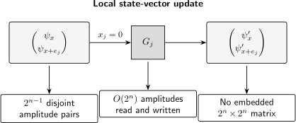
A one-qubit gate acts on $2^{n-1}$ disjoint amplitude pairs. Implementations stream those pairs through a small $2\times2$ kernel; they do not construct the embedded $2^n\times2^n$ matrix.

Why the full circuit matrix is usually wrong

The circuit unitary is a $2^n\times2^n$ matrix with $4^n$ complex entries. Constructing it explicitly throws away the main advantage of a local circuit description. If the goal is one output state, apply each local gate to a vector instead:

$$\lvert\psi_L\rangle = G_LG_{L-1}\cdots G_1 \lvert\psi_0\rangle.$$

For $L$ gates of bounded locality, a straightforward state-vector simulation uses

$$T=O(L2^n), \qquad M=O(2^n),$$

up to gate-specific constants and parallelization costs. Constructing the global unitary uses $O(4^n)$ memory before it is even applied. Full process or unitary reconstruction is appropriate only for small registers when the process itself is the requested output.

The Memory Wall

With double-precision real and imaginary parts, one complex amplitude commonly occupies 16 bytes. The state array alone then requires

$$M_{\mathrm{sv}}(n) = 16\times2^n\ \mathrm{bytes}.$$

Qubits	State-vector storage
20	16 MiB
25	512 MiB
30	16 GiB
35	512 GiB
40	16 TiB
45	512 TiB

These are lower bounds for one state vector. Alignment, work buffers, fused gates, checkpoints, distributed halos or partner buffers, observables, and runtime overhead require additional memory. A machine advertised with 16 GiB cannot safely be assumed to simulate an arbitrary 30-qubit state in double precision.

Each added qubit doubles both state storage and the work of a generic local gate. Parallel hardware improves the constant and increases available memory; it does not remove the exponential scaling. Conversely, qubit count alone does not determine difficulty for specialized methods. A thousand-qubit Clifford circuit or a low-entanglement one-dimensional circuit may be easy for a structured representation, while a much narrower generic circuit may saturate state-vector memory.

Worked Example: Bell-State Simulation

Start in $\lvert00\rangle$, apply $H$ to $Q_1$, then a controlled-NOT with $Q_1$ as control and $Q_2$ as target. In basis order $\lvert00\rangle,\lvert01\rangle,\lvert10\rangle,\lvert11\rangle$, the initial state is

$$\boldsymbol\psi_0 = \begin{pmatrix} 1&0&0&0 \end{pmatrix}^{\mathsf T}.$$

The Hadamard acts on pairs separated by $e_1=2$:

$$\boldsymbol\psi_1 = \frac{1}{\sqrt2} \begin{pmatrix} 1&0&1&0 \end{pmatrix}^{\mathsf T}.$$

The controlled-NOT permutes the amplitudes associated with $\lvert10\rangle$ and $\lvert11\rangle$, giving

$$\boldsymbol\psi_2 = \frac{1}{\sqrt2} \begin{pmatrix} 1&0&0&1 \end{pmatrix}^{\mathsf T}.$$

A terminal computational-basis measurement must therefore return 00 and 11 with probability $1/2$ each. If a simulator returns 01 and 10, the result often indicates a control-target or bit-order mismatch rather than a failure of quantum mechanics.

This tiny example tests initialization, one-qubit indexing, controlled-gate semantics, basis order, probability formation, and output-string formatting. Small analytic fixtures should be kept even in high-performance simulator test suites.

Measurement and Requested Outputs

Terminal sampling

For a final computational-basis measurement, the ideal distribution is

$$p(x)=|\psi_x|^2.$$

After one state evolution, a simulator can construct a cumulative or hierarchical probability data structure and draw many terminal samples without reapplying the circuit. Sampling cost and preprocessing depend on the chosen data structure. The output order still has to be translated from storage bits to declared classical-register bits.

Finite shots estimate rather than reveal the distribution. For a Bernoulli event with empirical frequency $\widehat p$, Hoeffding’s inequality gives

$$\Pr\!\left( |\widehat p-p|\geq\epsilon \right) \leq 2e^{-2N\epsilon^2}.$$

This sampling uncertainty is distinct from floating-point error and from any approximation made by the simulator.

Mid-circuit measurement

Suppose $Q_j$ is measured in the computational basis. The probability of outcome $m\in\{0,1\}$ is

$$p_m = \sum_{x:x_j=m} |\psi_x|^2.$$

For a sampled trajectory, draw $m$, zero amplitudes in the other branch, and renormalize:

$$\psi'_x = \begin{cases} \psi_x/\sqrt{p_m}, & x_j=m,\\ 0, & x_j\neq m. \end{cases}$$

The classical result must then be written to the declared classical register and may control later operations. A reset is not generally a unitary gate on the measured qubit; it can be implemented as measurement plus a conditional correction or as an explicit channel.

One trajectory produces one branch. Exact probabilities for all branches may require a branching tree whose width grows exponentially with the number of measurements. Repeating a dynamic circuit shot by shot can also require re-evolution after each branch point. Checkpointing, branch reuse, deferred measurement transformations, and classical-quantum state representations can reduce work in suitable circuits, but they must preserve the original outcome semantics.

Expectations and reduced states

If the requested output is an observable $O$, compute

$$\langle O\rangle = \langle\psi\rvert O\lvert\psi\rangle.$$

For a diagonal observable this is a weighted sum over $|\psi_x|^2$. For a Pauli string or other sparse local operator, apply a structured kernel and take an inner product. Constructing a dense $2^n\times2^n$ observable is normally as unnecessary as constructing the circuit unitary.

For a small subsystem $S$, the reduced state is

$$\rho_S = \operatorname{Tr}_{\bar S} \lvert\psi\rangle\langle\psi\rvert.$$

Its output has $4^{|S|}$ entries, but computing it from a generic full state still requires traversing the global amplitudes. Partial Trace owns the canonical subsystem algebra.

Method Families and Their Regimes

The best simulator depends on width, depth, gate structure, entanglement, non-Clifford resources, topology, requested output, and accuracy.

Method	Main representation	Favorable regime	Limiting resource
Schrödinger state vector	all $2^n$ amplitudes	generic gates, moderate width, many output queries	exponential memory and memory traffic
dense unitary or process	all $4^n$ matrix entries	tiny circuits requiring the full process	exponential-squared storage in Hilbert dimension
Feynman path sum	sums over intermediate alternatives	selected amplitudes and memory-constrained cuts	number of paths and cancellation
Schrödinger–Feynman hybrid	several smaller state vectors joined across cuts	circuits separable by a modest cut	cut count and repeated subproblems
stabilizer methods	generators or tableaux	Clifford circuits and related structured families	non-Clifford resources
tensor networks	tensors plus contraction plan	favorable topology, depth, and contraction width	contraction width and intermediate tensors
decision diagrams	shared graph of repeated amplitudes or operators	states and operations with strong redundancy	graph can lose compression abruptly
density matrices	$4^n$ operator entries	small noisy or mixed-state circuits	memory and runtime scale as $4^n$
stochastic trajectories	ensemble of pure-state runs	some open-system and dynamic tasks	trajectory variance and sample count

State vector versus path summation

The state-vector, or Schrödinger, method propagates the whole wavefunction layer by layer. Runtime is approximately linear in circuit size for fixed width, but memory is exponential in width. It is attractive when many amplitudes, observables, or samples are needed from the same final state.

A path-sum, or Feynman, method expands selected outputs over intermediate indices. It can use much less memory, but the number of terms can grow exponentially with depth, cuts, or entangling gates. The method is attractive when only a few amplitudes are requested or when a circuit can be cut into weakly connected pieces. Hybrid algorithms trade state-vector width against the number of cut assignments.

Structure is a computational resource

Efficient classical simulation of a restricted circuit does not imply that all circuits of the same width are easy. Stabilizer methods exploit algebraic closure of Clifford operations. Tensor networks exploit a favorable contraction graph or bounded entanglement representation. Decision diagrams exploit repeated substructure. Low-depth geometry, few non-Clifford gates, limited Schmidt rank, commuting structure, or a small separator may each be useful, but they are different resources.

Accordingly, report more than qubit count. At minimum include gate counts by type, depth, connectivity, measurement placement, non-Clifford content, contraction or cut information for structured methods, and the requested output. “Simulated 100 qubits” is not a meaningful performance claim without the circuit family and error contract.

Performance Engineering for State Vectors

The calculation is often bandwidth bound

A local gate reads and writes nearly the entire state vector. For small gate matrices, data movement can dominate arithmetic. Performance therefore depends on contiguous access, cache reuse, vector instructions, memory channels, and avoiding unnecessary copies. A mathematically sparse one- or two-qubit gate does not make the evolved state sparse in general.

The target wire controls stride. Under this page’s indexing convention, a gate on $Q_n$ updates adjacent amplitudes, whereas a gate on $Q_1$ pairs amplitudes separated by half the array. Cache blocking or an internal qubit permutation can improve locality. If storage order changes, measurement strings and every later gate must use the same mapping.

Gate fusion

Gate fusion combines several nearby operations into one small dense kernel. It can reduce complete passes through memory and amortize dispatch overhead. Fusion is not free: a fused $k$-qubit matrix has $4^k$ entries and each local group contains $2^k$ amplitudes. Excessive fusion increases arithmetic, register pressure, compilation time, and cache demand.

A correct fusion pass must preserve dependency order, classical-control boundaries, measurement semantics, parameter values, and the declared floating-point contract. Comparing a fused simulator only with its own fused output is not independent validation.

Threads, accelerators, and distributed memory

The disjoint amplitude groups of a local gate expose parallel work. CPUs can split groups across threads; GPUs can map them to many lanes; distributed systems can partition the state vector across ranks.

In distributed memory, some target bits are local to a rank and others select amplitudes stored on different ranks. A gate on a distributed bit requires partner exchange, transpose, or another communication strategy. The cost then depends on network bandwidth and latency as well as floating-point throughput. Reordering storage bits can cluster communication-heavy gates, but the logical wire permutation must remain explicit.

Strong scaling eventually saturates when communication, synchronization, or fixed overhead dominates. Weak scaling can look excellent while total resources still double for every added generic qubit. Performance reports should include state precision, memory footprint, circuit family, gate mix, number of nodes or accelerators, communication volume, initialization and I/O policy, and whether compilation and sampling time are included.

Batched simulation

Parameter sweeps, gradients, noisy trajectories, and test suites may require many related state vectors. Batching can reuse gate metadata and improve accelerator occupancy, but it multiplies state storage. Shared prefixes can be checkpointed, provided later branches do not mutate the shared state. A batched throughput claim should state the number of states and latency per circuit; aggregate gates per second can conceal poor single-circuit latency.

Numerical Accuracy

Unitary evolution preserves norm mathematically, but floating-point kernels accumulate roundoff. Useful diagnostics include

$$\epsilon_{\mathrm{norm}} = \left| 1-\langle\psi\vert\psi\rangle \right|$$

and a round-trip error obtained by applying $U_C$ and then $U_C^\dagger$. Renormalizing after every gate can hide an unstable or nonunitary kernel; norm should be monitored before any corrective normalization.

Two state vectors that differ only by global phase represent the same pure state. A phase-insensitive comparison uses

$$F = \left| \langle\phi\vert\psi\rangle \right|^2, \qquad D = \sqrt{1-F}.$$

For normalized pure states, $D$ is their trace distance and bounds differences in measurement statistics. Elementwise array comparison without phase alignment can falsely reject a correct result.

Single precision reduces memory and data traffic, sometimes substantially, but changes the error budget. Precision should be treated as a simulation parameter: compare against higher precision on representative circuits, track norm and conserved quantities, and test sensitivity as depth grows.

Approximate simulators introduce another error source. A mature result states whether the guarantee concerns state norm, fidelity, observable error, amplitude error, probability error, or total variation distance. A truncation tolerance internal to an algorithm is not automatically a bound on the reported physical quantity.

Dynamic Circuits and Classical Control

A dynamic simulator needs more than a state vector. Its runtime state includes

$$\mathcal S_t = \left( \lvert\psi_t\rangle, c_t, \ell_t, r_t \right),$$

where $c_t$ is the classical store, $\ell_t$ is the program location, and $r_t$ contains random-generator state or an explicit branch label. Conditions, loops, and subroutines read classical values according to the source language’s type and scope rules.

Important semantic questions include:

• whether measurement writes overwrite or append to a classical register;
• how bit arrays are converted to integers in conditions;
• whether uninitialized classical values are illegal;
• whether reset is a primitive channel or lowered sequence;
• how bounded and data-dependent loops terminate;
• whether random seeds identify one trajectory or an entire experiment;
• which operations are allowed after a qubit is measured or discarded;
• whether delays and timing affect the modeled result.

An ideal simulator may ignore physical duration while preserving operation order. A timing-aware or noisy simulator cannot. The target profile should say whether delays are semantic, whether simultaneous operations are grouped, and whether classical latency changes the channel being simulated.

A Reproducible Simulator Contract

A result should record enough information to reconstruct both the circuit and the simulator’s interpretation of it:

• source and lowered IR hashes, schema versions, and gate definitions;
• logical wire order, storage-bit order, displayed bitstring order, and classical-register layout;
• initial quantum and classical states;
• parameter values, units, and expression-evaluation precision;
• simulator method, implementation version, backend, and hardware;
• floating-point precision, fusion, qubit permutation, and parallel settings;
• measurement, reset, discard, and classical-control semantics;
• requested output and its ordering, normalization, and precision;
• random-number generator, seed hierarchy, shot count, and batching policy;
• all approximation, truncation, cut, or trajectory tolerances;
• runtime, peak memory, communication, and inclusion or exclusion of setup;
• validation fixtures, independent comparisons, and observed numerical error.

The output type should prevent invalid claims. A sample-only backend should not silently expose “exact probabilities” estimated from finite shots. An approximate tensor contraction should not label its state as exact. A state-vector backend should distinguish an amplitude array from a density matrix and identify its basis order.

Verification and Validation

A trustworthy simulator is tested in layers.

Algebraic unit tests

• Verify each primitive gate against its declared matrix and wire order.
• Check unitarity where required and trace preservation for channels.
• Test controlled gates for every control value and target basis state.
• Test parameter signs, angle units, and global-phase conventions.
• Check measurement probabilities and normalized post-measurement states.

Circuit-level invariants

• Identity and empty circuits preserve the input exactly.
• $U$ followed by $U^\dagger$ returns the initial state within tolerance.
• Norm and declared conserved quantities remain stable.
• SWAP networks and wire permutations give the expected output order.
• Bell and GHZ fixtures reproduce analytic correlations.
• Classically controlled corrections execute on the intended outcomes.

Independent differential tests

Compare small circuits with a separate implementation or with explicit dense matrix multiplication. Generate random unitary circuits at sizes where both methods are safe, and compare phase-insensitive state fidelity, selected amplitudes, probabilities, and samples. Independence matters: two backends that share the same parser, fusion pass, or gate table may share the same bug.

Statistical tests

For sampled outputs, expected count deviations scale with shot number. Use a predeclared goodness-of-fit or confidence procedure rather than requiring exact frequency equality. Test deterministic outcomes, balanced outcomes, rare events, correlated bitstrings, and mid-circuit branches. Fixing one random seed is useful for reproduction but not a statistical validation suite.

Scaling tests

Benchmark width, depth, gate locality, target-bit stride, gate mix, output type, and batch size separately. Report warm and cold execution if compilation, memory allocation, data transfer, or kernel caching matters. A benchmark made only of adjacent one-qubit gates does not characterize communication-heavy distributed simulation.

Choosing a Simulator

Use the least expensive method that answers the declared question with a defensible error statement.

Question	Good first choice
inspect all amplitudes of a moderate generic circuit	exact state vector
debug wire order and gate semantics	state vector plus tiny dense reference
sample many terminal shots after one ideal circuit	state vector, then repeated sampling
follow many mid-circuit branches	trajectory, branch reuse, or explicit classical-quantum representation
simulate a large Clifford circuit	stabilizer method
evaluate a low-entanglement or low-treewidth circuit	tensor-network method
compute a few amplitudes beyond state-vector memory	path, cut, or tensor contraction
model a small circuit with general noise	density matrix or channel propagation
model Markovian noise on a larger pure-state register	stochastic trajectories, with convergence checks
certify an approximate large-circuit result	cross-method checks and an output-level error contract

Method selection should be revisited when the requested output changes. A tensor contraction optimized for one amplitude may be poor for millions of samples. A state vector retained for many observables may be better than recontracting each observable. A density matrix that is convenient at twelve qubits becomes impossible long before a pure-state vector at the same precision.

Common Mistakes

• Building the $2^n\times2^n$ circuit matrix to compute one output state.
• Saying “exact simulation” without identifying floating precision and whether algorithmic truncation is absent.
• Treating bit order, wire order, storage order, and printed outcome order as interchangeable.
• Comparing state vectors elementwise without allowing a global phase.
• Reporting qubit count without circuit family, depth, gate mix, output task, accuracy, and hardware resources.
• Assuming a sparse gate implies a sparse state throughout the computation.
• Claiming that threads, GPUs, or distributed memory remove exponential scaling.
• Estimating “ideal probabilities” from finite samples when the exact state is already available.
• Reusing terminal-sampling logic for mid-circuit measurements without collapse and classical-state updates.
• Renormalizing silently and thereby hiding nonunitary numerical drift.
• Calling a truncation threshold an output-error bound without proving the connection.
• Validating two backends that share the same parser and gate implementation as if they were independent.
• Comparing simulator throughput while excluding different setup, communication, compilation, or sampling costs.
• Confusing a classically simulated circuit with a quantum simulator of a physical target model.

Exercises

1. Derive the one-qubit pair update

For $n=3$ with basis order $\lvert000\rangle,\ldots,\lvert111\rangle$, list the amplitude pairs updated by a gate on $Q_2$.

Solution

Here $e_2=2^{3-2}=2$. Choose indices whose $Q_2$ bit is zero. The pairs are

$$(0,2),\quad(1,3),\quad(4,6),\quad(5,7).$$

In bitstrings they are

$$(000,010),\quad(001,011),\quad (100,110),\quad(101,111).$$

Each pair is multiplied by the same $2\times2$ gate matrix, and the four pairs are disjoint.

2. Find a memory-limited qubit count

A node provides 256 GiB, but at least 25 percent must remain available for the runtime and work buffers. What is the largest double-complex state vector that fits under this policy?

Solution

The state may use at most $192$ GiB. A 33-qubit vector needs

$$16\times2^{33}\ \mathrm{bytes} = 128\ \mathrm{GiB},$$

while a 34-qubit vector needs $256$ GiB. Therefore the largest allowed vector has 33 qubits. This calculation does not guarantee good performance; it only checks the memory policy.

3. Compare vector and unitary storage

How much double-complex storage is required for a 15-qubit state vector and for the full 15-qubit unitary?

Solution

The state vector requires

$$16\times2^{15} = 524{,}288\ \mathrm{bytes} = 512\ \mathrm{KiB}.$$

The unitary requires

$$16\times4^{15} = 16\ \mathrm{GiB}.$$

The full matrix is $2^{15}=32{,}768$ times larger because it stores one output vector for every input basis vector.

4. Simulate a measurement collapse

The two-qubit state in basis order $00,01,10,11$ is

$$\lvert\psi\rangle = \frac{1}{\sqrt6} \left( \lvert00\rangle +\lvert01\rangle +2\lvert11\rangle \right).$$

Measure $Q_1$. Find both outcome probabilities and conditional states.

Solution

The $Q_1=0$ amplitudes have total probability

$$p_0 = \frac16+\frac16 = \frac13,$$

and the normalized state is

$$\lvert\psi_0\rangle = \frac{\lvert00\rangle+\lvert01\rangle}{\sqrt2}.$$

The $Q_1=1$ branch has probability $p_1=4/6=2/3$ and conditional state $\lvert\psi_1\rangle=\lvert11\rangle$.

5. Separate global phase from error

A reference state is $\lvert\phi\rangle$ and a simulator returns $\lvert\psi\rangle=-i\lvert\phi\rangle$. An elementwise difference is nonzero. What should a physical state comparison report?

Solution

The states differ only by global phase. Their overlap magnitude is one, so

$$F = |\langle\phi\vert\psi\rangle|^2 = 1, \qquad D=0.$$

A physical pure-state comparison should report agreement. If an application requires a phase relative to another coherent branch, that branch must be part of the simulated state rather than treated as an external global reference.

6. Distinguish strong and weak outputs

Backend A returns $p(0000)$ to additive error $10^{-8}$. Backend B returns bitstrings sampled from a distribution within total variation distance $10^{-3}$ of the target. Which is strong simulation and which is weak simulation?

Solution

Backend A performs a strong task because it estimates a specified output probability. Backend B performs a weak task because it samples from an approximately correct distribution. Neither contract automatically dominates the other: one accurate probability does not provide the full distribution, and sample access estimates rare probabilities inefficiently.

7. Identify distributed communication

A distributed state vector is partitioned so each rank owns contiguous blocks and the two most significant storage bits select the rank. Which one-qubit gates can be applied without exchanging amplitudes between ranks?

Solution

Gates on storage bits other than the two most significant bits pair amplitudes within each rank’s local block and need no inter-rank amplitude exchange. A gate on either rank-selecting bit pairs amplitudes held by different ranks and requires communication or a prior data-layout transformation. Logical wire labels may be permuted onto storage bits, but that mapping must remain explicit.

8. Design an independent validation fixture

You have written a fused state-vector backend. Propose a test that is more independent than comparing it with the same backend after disabling fusion.

Solution

For small random circuits, construct each embedded gate with a separate dense linear-algebra implementation, multiply the gates in declared time order, and apply the resulting matrix to the input. Compare the result with the fused backend using phase-insensitive fidelity and selected amplitudes. Use a separate gate table and index-embedding routine so parser, fusion, and kernel bugs are not shared. Analytic Bell, GHZ, SWAP, and inverse-circuit fixtures add interpretable failures.

9. Explain why terminal sampling is cheaper

Why can one ideal state-vector evolution produce many terminal measurement shots, while a dynamic circuit with feedforward may require repeated evolution?

Solution

Terminal measurement does not affect any later quantum operation. Once the final probabilities $|\psi_x|^2$ are available, arbitrarily many classical samples can be drawn from that fixed distribution. In a dynamic circuit, a mid-circuit outcome collapses the state and selects later operations. Different shots can follow different quantum branches, so later evolution generally has to be performed for each sampled branch unless checkpoints or shared branch structure can be reused exactly.

Research Status

Exact state-vector simulation and its shared-memory, accelerator, and distributed implementations are mature. Active engineering continues in cache blocking, gate fusion, communication avoidance, batching, mixed precision, and portable accelerator kernels. Performance remains hardware and circuit dependent; no single throughput number characterizes a simulator.

Specialized and hybrid simulation remain active research areas. Important directions include better tensor contraction and slicing, stabilizer-rank and Clifford-plus-non-Clifford decompositions, decision-diagram robustness, Schrödinger–Feynman tradeoffs, approximate sampling with auditable error, dynamic-circuit branch reuse, and distributed simulation across heterogeneous resources.

Classical simulation is indispensable for software testing and for validating quantum-hardware claims, but the baseline evolves. A claim of quantum advantage must compare against credible algorithms for the exact circuit ensemble, requested output, target fidelity, available classical resources, and total cost. Exponential state dimension alone is not such a comparison.

Further Connections

• Circuit Model defines the register, operation, measurement, classical-control, and resource semantics a simulator must execute.
• Digital Quantum Simulation concerns executing encoded physical dynamics on quantum hardware; the present page concerns classically simulating the resulting circuits.
• Circuit Intermediate Representations defines the typed input, capability profile, lowering provenance, and output-map metadata supplied to a backend.
• Quantum Software Stack places simulators beside compilers, target models, execution services, and reproducible result records.
• Stabilizer Simulation develops the polynomial Clifford-circuit backend, tableau and graph-state representations, repeated-shot Pauli-frame sampling, QEC detector streams, and decoder-facing validation.
• Tensor-Network Simulation develops MPS gate evolution, arbitrary spacetime contraction, path optimization, slicing, dynamic branches, sampling reuse, and approximation evidence.
• Noise Simulation binds channels, generators, leakage, correlations, and readout to compiled timelines and compares density, trajectory, Pauli, tensor, and memory-bearing engines under one uncertainty ledger.
• Cross-Entropy Benchmarking turns selected ideal output probabilities into a random-circuit score and specifies the simulator precision, compiled-reference, and evolving classical-baseline evidence that score requires.
• Verification of Quantum Advantage explains how exact, approximate, noisy, and verifier-targeting simulators define a dated classical frontier and can narrow an experimental advantage claim.
• Single-Qubit Gates and Multi-Qubit Gates own the gate matrices and semantic distinctions used by primitive kernels.
• Tensor Product Ordering develops the canonical translation between subsystem order, basis order, and matrix representations.
• Density Operators for Quantum Information develops mixed states, channels, reduced states, and measurement formulas needed by density-matrix simulation.
• Noise in Quantum Information distinguishes physical noise models from ideal-simulator roundoff and algorithmic approximation.
• Variational Quantum Algorithms explains how exact, sampled, noisy, and hardware objective evaluations enter an adaptive optimization and validation loop.
• What Is Quantum Simulation? develops digital, analog, and hybrid quantum emulation of target physical models.

References

1. M. A. Nielsen and I. L. Chuang, Quantum Computation and Quantum Information, 10th anniversary ed., Cambridge University Press (2010), doi:10.1017/CBO9780511976667.
2. R. P. Feynman, “Simulating physics with computers,” International Journal of Theoretical Physics 21, 467–488 (1982), doi:10.1007/BF02650179.
3. K. De Raedt et al., “Massively parallel quantum computer simulator,” Computer Physics Communications 176, 121–136 (2007), doi:10.1016/j.cpc.2006.08.007.
4. T. Jones, A. Brown, I. Bush, and S. C. Benjamin, “QuEST and high performance simulation of quantum computers,” Scientific Reports 9, 10736 (2019), doi:10.1038/s41598-019-47174-9.
5. T. Häner and D. S. Steiger, “0.5 petabyte simulation of a 45-qubit quantum circuit,” in Proceedings of SC17 (2017), doi:10.1145/3126908.3126947.
6. A. Fatima and I. L. Markov, “Faster Schrödinger-style simulation of quantum circuits,” in 2021 IEEE International Symposium on High-Performance Computer Architecture, 194–207 (2021), arXiv:2008.00216.
7. I. L. Markov and Y. Shi, “Simulating quantum computation by contracting tensor networks,” SIAM Journal on Computing 38, 963–981 (2008), doi:10.1137/050644756.
8. B. Villalonga et al., “A flexible high-performance simulator for verifying and benchmarking quantum circuits implemented on real hardware,” npj Quantum Information 5, 86 (2019), doi:10.1038/s41534-019-0196-1.
9. S. Aaronson and D. Gottesman, “Improved simulation of stabilizer circuits,” Physical Review A 70, 052328 (2004), doi:10.1103/PhysRevA.70.052328.
10. S. Bravyi and D. Gosset, “Improved classical simulation of quantum circuits dominated by Clifford gates,” Physical Review Letters 116, 250501 (2016), doi:10.1103/PhysRevLett.116.250501.
11. M. Van den Nest, “Classical simulation of quantum computation, the Gottesman–Knill theorem, and slightly beyond,” Quantum Information and Computation 10, 258–271 (2010), arXiv:0811.0898.