Multi-Qubit Gates

Short Definition

A multi-qubit gate is a joint operation on two or more qubits. An ideal $k$-qubit unitary is a matrix

$$U\in U(2^k), \qquad U^\dagger U=I,$$

defined relative to an ordered tensor-product basis. Common families include:

• controlled gates such as CNOT and CZ;
• exchange gates such as SWAP and iSWAP;
• multiply controlled gates such as Toffoli;
• continuously parameterized interactions generated by two-qubit Hamiltonians.

Some multi-qubit primitives are measurements rather than unitaries. A parity measurement, for example, projects onto an even or odd subspace while ideally preserving coherence inside that subspace.

This page is the canonical home for common multi-qubit gates, their exact basis actions, entangling capability, and the distinction between logical, native, compiled, and measured operations. Operators on Composite Systems owns the tensor-product algebra, Bell States owns the resulting maximally entangled states, and Circuit Model owns wire order, composition, and resource accounting.

Fix the Ordered Basis

For two qubits labeled $A$ and $B$, this page uses

$$\mathcal H_{AB} = \mathcal H_A\otimes\mathcal H_B$$

with computational basis order

$$\lvert00\rangle,\quad \lvert01\rangle,\quad \lvert10\rangle,\quad \lvert11\rangle.$$

The first bit labels $A$ and the second labels $B$. A matrix, a circuit diagram, and a bitstring returned by software agree only after their ordering conventions are matched. Tensor Product Ordering is the convention anchor.

A gate acting independently on the factors has the form

$$U_A\otimes V_B.$$

A general joint gate need not factor this way. “Two-qubit gate” describes support, not entangling ability: SWAP acts jointly but never entangles a product input, while CNOT can entangle some product inputs but not others.

Controlled Unitaries

Let $A$ be the control and $B$ the target. The controlled version of a one-qubit unitary $U$ is

$$C_A(U_B) = \lvert0\rangle\langle0\rvert_A\otimes I_B + \lvert1\rangle\langle1\rvert_A\otimes U_B.$$

In the stated basis, it has block form

$$C(U) = \begin{pmatrix} I&0\\ 0&U \end{pmatrix}.$$

The control is not measured. If it is in a superposition, the two control sectors evolve coherently and can become entangled with the target. Controlled Operations develops the semantic and evidence audit for projector-controlled blocks, open and multiple controls, multiplexed branches, branch-relative phases, and licensed access. Here the definition fixes the common gate families; Algorithmic Primitives owns oracle uses, and Gate Decomposition owns synthesis.

Global phases cannot be discarded before adding a control. If $V=e^{i\gamma}U$, then

$$C(V) = \left[ P_A(\gamma)\otimes I_B \right] C(U),$$

so the phase becomes relative between the control sectors. Single-Qubit Gates gives the full phase analysis.

Controlled-NOT

The controlled-NOT gate, written CNOT, CX, or $C(X)$, acts as

$$\operatorname{CNOT}_{A\to B} \lvert a,b\rangle = \lvert a,b\oplus a\rangle,$$

where $a,b\in\{0,1\}$ and $\oplus$ is addition modulo two. Its matrix is

$$\operatorname{CNOT}_{A\to B} = \begin{pmatrix} 1&0&0&0\\ 0&1&0&0\\ 0&0&0&1\\ 0&0&1&0 \end{pmatrix}.$$

The first qubit controls the second. Reversing control and target gives a different matrix:

$$\operatorname{CNOT}_{B\to A} \lvert a,b\rangle = \lvert a\oplus b,b\rangle.$$

Entanglement from coherent control

On the product input $\lvert+\rangle_A\lvert0\rangle_B$,

$$\begin{aligned} \operatorname{CNOT}_{A\to B} \lvert+0\rangle &= \frac{ \lvert00\rangle+\lvert11\rangle }{\sqrt2} \\ &= \lvert\Phi^+\rangle. \end{aligned}$$

The output is maximally entangled. Yet CNOT does not entangle every product state: each computational-basis input remains a computational-basis product state.

CNOT is not a cloning gate

For an unknown state

$$\lvert\psi\rangle = \alpha\lvert0\rangle+\beta\lvert1\rangle,$$

CNOT with a blank target gives

$$\operatorname{CNOT} \left( \lvert\psi\rangle\lvert0\rangle \right) = \alpha\lvert00\rangle + \beta\lvert11\rangle.$$

This is generally entangled and is not

$$\lvert\psi\rangle\otimes\lvert\psi\rangle.$$

CNOT coherently copies a known computational-basis label. It does not clone an arbitrary quantum state.

Controlled-Z

The controlled-$Z$ gate applies a minus sign only to $\lvert11\rangle$:

$$\operatorname{CZ} = \operatorname{diag}(1,1,1,-1).$$

Equivalently,

$$\operatorname{CZ}\lvert a,b\rangle = (-1)^{ab} \lvert a,b\rangle.$$

Unlike the usual CNOT diagram, CZ is symmetric under exchanging the two qubits. Either qubit can be described as the control because the matrix depends only on the product $ab$.

CNOT and CZ have the same nonlocal content. Hadamard conjugation on the target gives

$$\begin{aligned} \operatorname{CZ} &= (I\otimes H) \\ &\quad\times \operatorname{CNOT}_{A\to B} (I\otimes H), \\ \operatorname{CNOT}_{A\to B} &= (I\otimes H) \\ &\quad\times \operatorname{CZ} (I\otimes H). \end{aligned}$$

Thus they are locally equivalent. Which one is cheaper depends on the native interaction, calibration, connectivity, and surrounding circuit.

On $\lvert++\rangle$, CZ produces

$$\operatorname{CZ}\lvert++\rangle = \frac{ \lvert00\rangle+\lvert01\rangle +\lvert10\rangle-\lvert11\rangle }{2},$$

a maximally entangled two-qubit graph state.

SWAP

SWAP exchanges the states assigned to two labeled subsystems:

$$\operatorname{SWAP} \lvert a,b\rangle = \lvert b,a\rangle.$$

Its matrix is

$$\operatorname{SWAP} = \begin{pmatrix} 1&0&0&0\\ 0&0&1&0\\ 0&1&0&0\\ 0&0&0&1 \end{pmatrix}.$$

For arbitrary product states,

$$\operatorname{SWAP} \left( \lvert\psi\rangle_A \otimes \lvert\phi\rangle_B \right) = \lvert\phi\rangle_A \otimes \lvert\psi\rangle_B.$$

The output remains a product state, so SWAP has zero entangling capability. It is nevertheless not a product unitary $U_A\otimes V_B$; it transfers the two unknown subsystem states jointly. This is the standard warning that nonlocal and entangling are not synonyms.

An ideal decomposition is

$$\begin{aligned} \operatorname{SWAP} &= \operatorname{CNOT}_{A\to B} \\ &\quad\times \operatorname{CNOT}_{B\to A} \operatorname{CNOT}_{A\to B}. \end{aligned}$$

Read right to left as a matrix product. The corresponding circuit applies the same three gates from left to right because the first and last factors are identical. A compiler may choose a different decomposition when the hardware has a native exchange interaction or when qubit relabeling can replace a physical move.

iSWAP and Exchange Gates

This page defines

$$\begin{aligned} \operatorname{iSWAP} \lvert01\rangle &= i\lvert10\rangle, \\ \operatorname{iSWAP} \lvert10\rangle &= i\lvert01\rangle. \end{aligned}$$

while leaving $\lvert00\rangle$ and $\lvert11\rangle$ unchanged. Its matrix is

$$\operatorname{iSWAP} = \begin{pmatrix} 1&0&0&0\\ 0&0&i&0\\ 0&i&0&0\\ 0&0&0&1 \end{pmatrix}.$$

With this sign convention,

$$\operatorname{iSWAP} = \exp\left[ \frac{i\pi}{4} \left( X\otimes X+Y\otimes Y \right) \right].$$

A Hamiltonian with the opposite sign generates the conjugate phase, often called $-\operatorname{iSWAP}$ or $\operatorname{iSWAP}^\dagger$ depending on notation. The matrix must accompany the name.

iSWAP is not merely SWAP times one global phase: the exchanged one-excitation states acquire $i$, while the zero- and two-excitation states do not. It can entangle product inputs. For example,

$$\begin{aligned} \operatorname{iSWAP}\lvert++\rangle &= \frac12 \left( \lvert00\rangle+i\lvert01\rangle \right. \\ &\qquad\left. + i\lvert10\rangle+\lvert11\rangle \right). \end{aligned}$$

which is maximally entangled.

Exchange-like interactions naturally produce continuous families such as

$$U_{XY}(\theta) = \exp\left[ -\frac{i\theta}{2} \left( X\otimes X+Y\otimes Y \right) \right],$$

with angle and sign conventions that vary across platforms and software. Fractional exchange gates, including square-root variants, can be native entanglers even when a full SWAP is not the desired logical operation.

Toffoli Gate

The Toffoli gate is a controlled-controlled-NOT on three ordered qubits:

$$\operatorname{CCNOT} \lvert a,b,c\rangle = \lvert a,b,c\oplus ab\rangle.$$

It flips the target $c$ only when both controls equal one. On computational-basis states it implements a reversible classical Boolean operation, but on superpositions it is a coherent quantum gate and can create entanglement. For example,

$$\begin{aligned} \operatorname{CCNOT} \left( \lvert+\rangle\lvert1\rangle\lvert0\rangle \right) &= \frac{ \lvert010\rangle+\lvert111\rangle }{\sqrt2}. \end{aligned}$$

The second qubit factors as $\lvert1\rangle$, while the first and third are entangled.

A Toffoli symbol in an algorithm does not imply a native three-body interaction. It is usually compiled into one- and two-qubit gates, possibly with clean or dirty ancillas. Exact gate counts depend on the basis set, connectivity, allowed relative phases, ancilla budget, and whether only a specific input subspace matters. A relative-phase Toffoli is not an exact Toffoli, even when it suffices inside a larger construction.

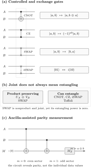
Common joint primitives separate into controlled, exchange, and measurement operations. SWAP is joint but product preserving; CNOT, CZ, iSWAP, and Toffoli can entangle suitable product inputs. In the parity circuit, two CNOTs write $a\oplus b$ onto an ancilla without revealing which basis state occurred inside the even or odd sector.

Entangling Capability

Capability is an existence statement

A two-qubit unitary $U$ is entangling if there exists at least one product input

$$\lvert\alpha\rangle_A \otimes \lvert\beta\rangle_B$$

whose output is entangled. It need not entangle every product input.

For a pure two-qubit output

$$\lvert\Psi\rangle = \sum_{a,b=0}^{1} c_{ab}\lvert a,b\rangle,$$

form the coefficient matrix

$$C= \begin{pmatrix} c_{00}&c_{01}\\ c_{10}&c_{11} \end{pmatrix}.$$

The state is product exactly when

$$\det C=0.$$

This gives a quick gate test on a chosen input. It does not characterize the gate on all inputs.

Operation	Product preserving for every input?	Can create entanglement?
$U_A\otimes V_B$	yes	no
SWAP	yes	no
CNOT	no	yes
CZ	no	yes
iSWAP	no	yes
Toffoli	no, across suitable three-qubit splits	yes

Local equivalence

Two two-qubit unitaries have the same nonlocal content when they differ only by local pre- and post-rotations:

$$U' = (u_A\otimes u_B) U (v_A\otimes v_B).$$

Local gates cannot create or destroy bipartite entanglement, so locally equivalent gates have the same optimal entangling capability. CNOT and CZ are the elementary example. iSWAP belongs to a different local-equivalence class even though it is also a perfect entangler.

SWAP supplies the important caveat: a gate may be nonproduct and operationally nonlocal while mapping every product state to another product state. Quantities based only on entanglement generated from product inputs assign SWAP zero even though it cannot be implemented as independent local unitaries.

Entangling power is a defined metric

In the technical literature, entangling power often means an average

$$e_p(U) = \int d\alpha\,d\beta\, E\left[ U \left( \lvert\alpha\rangle \otimes \lvert\beta\rangle \right) \right],$$

where $E$ is an entanglement measure and the integral uses a stated ensemble of product inputs. A numerical value is meaningless unless the measure, input distribution, and normalization are specified. “Can entangle,” “can create a maximally entangled state,” “has nonzero average entangling power,” and “is costly on a device” are four different claims.

Parity Measurements

A two-qubit $Z$-parity measurement measures the observable

$$Z_AZ_B = Z_A\otimes Z_B.$$

Its projectors are

$$\begin{aligned} \Pi_{\mathrm{even}} &= \frac{I+Z_AZ_B}{2}, \\ \Pi_{\mathrm{odd}} &= \frac{I-Z_AZ_B}{2}. \end{aligned}$$

The even subspace is spanned by $\lvert00\rangle,\lvert11\rangle$ and has eigenvalue $+1$. The odd subspace is spanned by $\lvert01\rangle,\lvert10\rangle$ and has eigenvalue $-1$.

An ancilla implementation initializes $M$ in $\lvert0\rangle$, applies

$$\operatorname{CNOT}_{A\to M} \quad\text{and}\quad \operatorname{CNOT}_{B\to M},$$

then measures $M$ in the computational basis. For a basis input $\lvert a,b\rangle$, the ancilla records

$$m=a\oplus b.$$

The ideal outcome-resolved state update is

$$\rho \longmapsto \frac{ \Pi_m\rho\Pi_m }{ \operatorname{Tr}(\rho\Pi_m) },$$

where $\Pi_0=\Pi_{\mathrm{even}}$ and $\Pi_1=\Pi_{\mathrm{odd}}$.

Coarse parity is not two separate readouts

An ideal parity measurement reveals only even versus odd. It preserves coherence within the selected subspace. For example,

$$\lvert\Phi^+\rangle = \frac{ \lvert00\rangle+\lvert11\rangle }{\sqrt2}$$

has even parity with certainty and is unchanged by an ideal nondemolition parity measurement.

Measuring $Z_A$ and $Z_B$ separately reveals whether the state was $\lvert00\rangle$ or $\lvert11\rangle$ and therefore destroys their coherence. Forgetting the two fine-grained records afterward does not undo that disturbance. The distinction is essential in stabilizer readout and measurement-induced entanglement.

A parity measurement is not a unitary gate on the data alone. It is an instrument with a classical outcome and a conditional state update. Hardware may realize it through an ancilla circuit, a shared resonator, a detector coupling, or another native joint measurement. Quantum Instruments owns the general formalism.

Pauli Group and Stabilizers treats signed Hermitian Pauli strings as algebraic checks and audits their common sectors and commutation signatures; this page retains outcome-resolved parity instruments and their elementary ancilla circuits. Syndrome Measurement owns signed stabilizer-check protocols, ordered circuit-fault propagation, repeated outcomes, and detector-record construction.

Native, Compiled, and Routed Gates

A circuit symbol names a logical operation. Hardware evolves under a platform-specific Hamiltonian and control schedule. Common idealized interactions include

$$\begin{aligned} U_{ZZ}(\theta) &= \exp\left( -\frac{i\theta}{2}Z\otimes Z \right), \\ U_{XX}(\theta) &= \exp\left( -\frac{i\theta}{2}X\otimes X \right), \\ G_{XY} &= X\otimes X+Y\otimes Y, \\ U_{XY}(\theta) &= \exp\left( -\frac{i\theta}{2}G_{XY} \right). \end{aligned}$$

Local rotations and echoed segments can convert these interactions into CNOT-like, CZ-like, or exchange-like logical gates. The same CNOT symbol may therefore mean:

1. a native calibrated instruction;
2. a short composite pulse sequence;
3. a CZ plus local Hadamards;
4. an interaction gate plus several frame changes;
5. a logical operation synthesized fault tolerantly.

Those implementations need not have the same duration, leakage, crosstalk, directionality, or error channel.

Connectivity also matters. If two logical qubits are not adjacent in the coupling graph, a compiler may route their states using SWAPs, teleportation-based primitives, movable carriers, or dynamic relabeling. Reporting only the abstract CNOT count can hide the dominant routing cost.

Resource claims need a contract

When comparing decompositions, state:

• the exact target, including allowed global or relative phases;
• the native gate alphabet and continuous parameters;
• directed or undirected connectivity;
• whether parallel gates are allowed;
• ancilla number, initialization, and reset assumptions;
• whether measurement and feedforward are available;
• the error metric and approximation tolerance;
• whether counts are logical, compiled, scheduled, or physical.

“Toffoli costs six CNOTs” or “SWAP costs three CNOTs” is a statement inside one ideal gate model, not a hardware-independent law.

Common Mistakes

• Comparing two-qubit matrices without fixing basis and tensor-factor order.
• Reversing CNOT control and target.
• Treating a coherent control wire as a classical if-statement.
• Saying CNOT clones an arbitrary qubit because it copies basis labels.
• Assuming every joint or nonlocal gate is entangling; SWAP is the counterexample.
• Treating iSWAP and SWAP as equal up to one global phase.
• Ignoring the sign convention in an exchange-generated iSWAP.
• Calling CZ directional even though its ideal matrix is symmetric.
• Replacing a parity measurement by separate one-qubit measurements and then discarding the extra records.
• Dropping a one-qubit gate phase before constructing its controlled version.
• Equating a logical gate symbol with one calibrated pulse.
• Quoting gate counts without connectivity, ancilla, phase, or tolerance assumptions.

Exercises

1. CNOT on a general state

Apply $\operatorname{CNOT}_{A\to B}$ to

$$\begin{aligned} \lvert\psi\rangle &= c_{00}\lvert00\rangle +c_{01}\lvert01\rangle \\ &\quad+ c_{10}\lvert10\rangle +c_{11}\lvert11\rangle. \end{aligned}$$

Solution

The control-zero amplitudes are unchanged. In the control-one sector, the target labels are exchanged:

$$\begin{aligned} \operatorname{CNOT}_{A\to B} \lvert\psi\rangle &= c_{00}\lvert00\rangle +c_{01}\lvert01\rangle \\ &\quad+ c_{10}\lvert11\rangle +c_{11}\lvert10\rangle. \end{aligned}$$

This also shows why reversing control and target changes the coordinate matrix.

2. Coherent copying and no-cloning

Show that CNOT maps $\lvert+0\rangle$ to a Bell state. Explain why the result is not two copies of $\lvert+\rangle$.

Solution

Linearity and the two relevant basis-state mappings give

$$\operatorname{CNOT}\lvert+0\rangle = \frac{ \lvert00\rangle+\lvert11\rangle }{\sqrt2}.$$

This is $\lvert\Phi^+\rangle$, whose one-qubit reduced states are maximally mixed. Two copies would be

$$\lvert+\rangle\lvert+\rangle = \frac{ \lvert00\rangle+\lvert01\rangle +\lvert10\rangle+\lvert11\rangle }{2},$$

a product state. CNOT copied the computational-basis branch label into correlations; it did not clone the superposition.

3. Convert CNOT to CZ

Prove

$$\operatorname{CZ} = (I\otimes H) \operatorname{CNOT}_{A\to B} (I\otimes H)$$

using the controlled-unitary form rather than multiplying $4\times4$ matrices.

Solution

Write

$$\begin{aligned} \operatorname{CNOT}_{A\to B} &= \lvert0\rangle\langle0\rvert_A \otimes I_B \\ &\quad+ \lvert1\rangle\langle1\rvert_A \otimes X_B. \end{aligned}$$

Conjugating the target by $H$ gives

$$\begin{aligned} &(I\otimes H) \operatorname{CNOT} (I\otimes H) \\ &= \lvert0\rangle\langle0\rvert \otimes I \\ &\quad+ \lvert1\rangle\langle1\rvert \otimes H X H \\ &= \lvert0\rangle\langle0\rvert \otimes I \\ &\quad+ \lvert1\rangle\langle1\rvert \otimes Z \\ &= \operatorname{CZ}. \end{aligned}$$

The identity $HXH=Z$ is the one-qubit basis change.

4. Decompose SWAP

Track bits through

$$\operatorname{CNOT}_{A\to B}, \quad \operatorname{CNOT}_{B\to A}, \quad \operatorname{CNOT}_{A\to B}$$

and show that the sequence implements SWAP. Why does this not contradict the fact that each CNOT can entangle?

Solution

Starting from $(a,b)$, the successive labels are

$$\begin{aligned} (a,b) &\longmapsto (a,a\oplus b) \\ &\longmapsto (b,a\oplus b) \\ &\longmapsto (b,a). \end{aligned}$$

Thus the composite is SWAP on every computational-basis state and therefore, by linearity, on every input.

Entangling capability is not additive gate by gate. Intermediate states may be entangled and later disentangled. The exact three-gate product maps every product input to the exchanged product state.

5. Test iSWAP entanglement

Use the coefficient-matrix criterion to show that $\operatorname{iSWAP}\lvert++\rangle$ is maximally entangled.

Solution

The output coefficient matrix is

$$C = \frac12 \begin{pmatrix} 1&i\\ i&1 \end{pmatrix}.$$

Its determinant is

$$\det C = \frac{ 1-i^2 }{4} = \frac12,$$

so the state is not product. For a normalized pure two-qubit state, the concurrence is

$$\mathcal C=2\lvert\det C\rvert=1.$$

Therefore the output is maximally entangled. The conclusion depends on the matrix convention for iSWAP, although changing all $i$ signs by complex conjugation leaves this entanglement value unchanged.

6. Preserve parity coherence

Compare an ideal $Z_AZ_B$ parity measurement with separate $Z_A$ and $Z_B$ measurements on $\lvert\Phi^+\rangle$.

Solution

Both components of

$$\lvert\Phi^+\rangle = \frac{ \lvert00\rangle+\lvert11\rangle }{\sqrt2}$$

have even parity. Hence

$$\Pi_{\mathrm{even}} \lvert\Phi^+\rangle = \lvert\Phi^+\rangle, \qquad \Pi_{\mathrm{odd}} \lvert\Phi^+\rangle = 0.$$

The ideal parity outcome is certainly even and the coherent Bell state is preserved.

Separate computational-basis measurements return $00$ or $11$, each with probability $1/2$. If those records are ignored, the state is

$$\rho = \frac12 \left( \lvert00\rangle\langle00\rvert + \lvert11\rangle\langle11\rvert \right),$$

with no off-diagonal coherence. Coarse-graining classical records after a finer measurement is not equivalent to performing the coarse quantum measurement.

7. Toffoli as an entangler

Apply Toffoli to $\lvert+\rangle\lvert1\rangle\lvert0\rangle$ and compute the reduced state of the first qubit.

Solution

The output is

$$\frac{ \lvert010\rangle+\lvert111\rangle }{\sqrt2} = \lvert1\rangle_B \otimes \frac{ \lvert00\rangle+\lvert11\rangle }{\sqrt2}_{AC}.$$

Tracing out $B$ and $C$ gives

$$\rho_A = \frac12 \left( \lvert0\rangle\langle0\rvert + \lvert1\rangle\langle1\rvert \right) = \frac I2.$$

The full state is pure while $\rho_A$ is mixed, so $A$ is entangled with $C$. The second control remains a product factor.

Where to Go Next

• Single-Qubit Gates fixes one-qubit matrices, rotation signs, phase conventions, and Euler synthesis.
• Circuit Model defines gate embedding, time order, dynamic circuits, and resource counts.
• Reversible Computation uses Toffoli and Fredkin as reversible classical primitives while tracking constants, garbage, and uncomputation; this page retains their gate actions, entangling behavior, and compilation caveats.
• Universal Gate Sets explains which local and entangling families are exactly or approximately universal.
• Gate Decomposition develops controlled-unitary constructions, Cartan/KAK synthesis, native local equivalence, Pauli rotations, and generic multiqubit reductions.
• Qubit Mapping and Routing explains how SWAPs, bridges, direction corrections, physical transport, and teleportation legalize multi-qubit interactions on constrained hardware.
• Pulse-Level Control binds native entangling semantics to calibrated concurrent controls, timing resources, crosstalk context, and executable pulse records.
• Operators on Composite Systems supplies local embeddings, product operators, and controlled block forms.
• Tensor Product Ordering prevents control-target and basis-index reversals.
• Bell States develops the maximally entangled outputs used in the examples.
• Quantum Teleportation combines an inverse Bell transform, two measurements, classical feed-forward, and Pauli corrections into an identity channel.
• Superdense Coding uses local Pauli encoding followed by the same inverse Bell transform to decode two classical bits.
• Local Unitary Equivalence treats state equivalence under independent subsystem rotations.
• Quantum Instruments gives the outcome-resolved framework for parity measurements.
• Quantum Gates Formula Card and Quantum Gates Reference Table provide compact lookup forms.
• Quantum Information Roadmap places multi-qubit gates before universality, algorithms, and error correction.

References

• M. A. Nielsen and I. L. Chuang, Quantum Computation and Quantum Information, 10th anniversary ed., Cambridge University Press, 2010, doi:10.1017/CBO9780511976667.
• A. Barenco, C. H. Bennett, R. Cleve, D. P. DiVincenzo, N. Margolus, P. Shor, T. Sleator, J. A. Smolin, and H. Weinfurter, “Elementary gates for quantum computation,” Physical Review A 52, 3457–3467, 1995, doi:10.1103/PhysRevA.52.3457.
• T. Toffoli, “Reversible computing,” in Automata, Languages and Programming, Lecture Notes in Computer Science 85, Springer, 1980, doi:10.1007/3-540-10003-2_104.
• P. Zanardi, C. Zalka, and L. Faoro, “Entangling power of quantum evolutions,” Physical Review A 62, 030301(R), 2000, doi:10.1103/PhysRevA.62.030301.
• N. Schuch and J. Siewert, “Natural two-qubit gate for quantum computation using the XY interaction,” Physical Review A 67, 032301, 2003, doi:10.1103/PhysRevA.67.032301.
• Y. Makhlin, “Nonlocal properties of two-qubit gates and mixed states, and the optimization of quantum computations,” Quantum Information Processing 1, 243–252, 2002, doi:10.1023/A:1022144002391.
• D. Ristè, M. Dukalski, C. A. Watson, G. de Lange, M. J. Tiggelman, Ya. M. Blanter, K. W. Lehnert, R. N. Schouten, and L. DiCarlo, “Deterministic entanglement of superconducting qubits by parity measurement and feedback,” Nature 502, 350–354, 2013, doi:10.1038/nature12513.
• D. P. DiVincenzo, “The physical implementation of quantum computation,” Fortschritte der Physik 48, 771–783, 2000, doi:10.1002/1521-3978(200009)48:9/11%3C771::AID-PROP771%3E3.0.CO;2-E.
• J. Preskill, Lecture Notes for Physics 219/Computer Science 219: Quantum Computation, Chapter 5, California Institute of Technology, course materials.