Pulse-Level Control

Short Definition

Pulse-level control is the target-specific lowering layer that turns an operation such as a rotation, entangling gate, reset, or measurement into a timed program of frame updates, waveform plays, waits, acquisitions, and classical events on named physical resources.

The output is not merely an array of voltage samples. A trustworthy pulse program states:

• which physical qubits, modes, ports, and shared resources it addresses;
• which rotating-frame, carrier, phase, sign, unit, and tensor-order conventions give the samples meaning;
• which calibration record and target epoch bind an abstract operation to a waveform family;
• how analytic envelopes are sampled, quantized, aligned, filtered, and scheduled;
• what computational subspace, leakage model, and simultaneous-operation context were assumed;
• how the resulting operation was simulated, measured, validated, and given a validity interval.

This page owns that representation and lowering contract. Rabi and Ramsey Control owns the canonical two-level experiments. Optimal Control owns GRAPE, Krotov, robust objectives, and related search methods. Control, Readout, and Calibration owns the physical delivery and observation chain, estimands, and tune-up experiments. Calibration Loops owns dependency-aware maintenance, drift monitoring, candidate acceptance, publication, and rollback. The task here is to connect those physical and experimental facts to an executable compiler artifact without pretending that a gate name uniquely determines a pulse.

The Lowering Contract

Let $G(\lambda)$ denote a parameterized operation with semantic parameters $\lambda$, let $\mathcal T$ be a target profile, and let $\kappa_\tau$ be a calibration snapshot valid near epoch $\tau$. Pulse lowering should be read as a typed transformation

$$\begin{aligned} \operatorname{Lower}_{\mathrm{pulse}} \bigl(G(\lambda),\mathcal T,\kappa_\tau,C\bigr) \longrightarrow \bigl(P,\Gamma\bigr), \end{aligned}$$

where $C$ is the execution context, $P$ is a pulse program, and $\Gamma$ is a certificate carrying provenance and validation claims. The context can include neighbor states, allowed concurrency, preceding frame state, thermal or motional preparation, and the required measurement basis. Two calls with the same gate name but different physical qubits, epochs, or contexts need not produce the same $P$.

The intended semantic statement has the form

$$\left. \mathcal E_{P,\mathcal T,\kappa_\tau,C} \right|_{\mathcal C} \approx_{\epsilon,M} \mathcal U_{G(\lambda)},$$

where $\mathcal C$ is the declared computational subspace, $M$ is a comparison metric, and $\epsilon$ is a tolerance. This notation deliberately exposes four facts:

1. the implemented object is generally a channel $\mathcal E$, not an ideal unitary;
2. restricting attention to $\mathcal C$ can hide leakage and return dynamics;
3. approximation is meaningless without a metric and tolerance;
4. the claim is conditional on a target, calibration state, and context.

A pulse definition is therefore closer to a versioned implementation of an interface than to a timeless identity. Gate Decomposition chooses a target operation alphabet. Pulse lowering binds an operation in that alphabet to physical controls.

Controlled Dynamics

Drift and control generators

A common finite-dimensional model is

$$H(t;\theta) = H_0(\theta) + \sum_{k=1}^{K} u_k(t)H_k(\theta),$$

where $H_0$ is the drift Hamiltonian, $H_k$ are control generators, $u_k(t)$ are real control functions, and $\theta$ collects device parameters. In a closed model, the propagator satisfies

$$i\hbar\frac{dU(t)}{dt} = H(t)U(t), \qquad U(0)=I,$$

and hence

$$U(T) = \mathcal T \exp\!\left[ -\frac{i}{\hbar} \int_0^T H(t)\,dt \right].$$

The time-ordering symbol $\mathcal T$ matters whenever Hamiltonians at different times fail to commute. Equal pulse areas then need not imply equal gates. Shape, order, detuning, and concurrent controls can all matter.

For an open model one may instead propagate

$$\frac{d\rho}{dt} = -\frac{i}{\hbar}[H(t),\rho] + \sum_j \gamma_j(t) \mathcal D[L_j]\rho,$$

with

$$\mathcal D[L]\rho = L\rho L^\dagger - \frac{1}{2} \left\{ L^\dagger L,\rho \right\}.$$

This Markovian form is useful but not universal. Colored noise, drift, state-dependent electronics, coherent spectators, and non-Markovian environments may require a larger model. Quantum Channels and Noise owns the channel formalism; the pulse artifact must identify which model was actually used.

A control model is not the device

The matrices $H_k$ are inferred approximations. Their coefficients can depend on drive amplitude, frequency, bias, neighboring excitations, and earlier pulses. Truncating an oscillator or motional Hilbert space can also change the predicted optimum. A waveform optimized against $H(t;\hat\theta)$ is a hypothesis about an implementation, not evidence that the laboratory realizes the target channel.

That distinction is central at pulse level because apparently small modeling choices move into the executable itself. The model version, basis truncation, parameter uncertainty, and transfer-function assumptions belong in $\Gamma$.

Carriers, Quadratures, and Frames

Fix an I/Q convention

One common real carrier convention is

$$s(t) = I(t)\cos(\omega_{\mathrm{LO}}t) - Q(t)\sin(\omega_{\mathrm{LO}}t) = \operatorname{Re} \left[ \varepsilon(t)e^{i\omega_{\mathrm{LO}}t} \right],$$

with complex envelope

$$\varepsilon(t)=I(t)+iQ(t).$$

Other sign and phase conventions are equally usable. They are not interchangeable. Mixer wiring, Fourier-transform conventions, local-oscillator phase, and software definitions can reverse the meaning of $Q$ or of a positive phase shift. A pulse IR must declare the convention or bind it to a versioned target profile.

Rotating-frame reduction

Consider the laboratory-frame two-level model

$$\frac{H_{\mathrm{lab}}(t)}{\hbar} = \frac{\omega_q}{2}\sigma_z + \Omega(t) \cos(\omega_d t+\phi) \sigma_x.$$

With the rotating-frame transformation

$$R(t)=e^{-i\omega_d t\sigma_z/2}, \qquad \lvert\psi_{\mathrm{rot}}\rangle = R^\dagger(t) \lvert\psi_{\mathrm{lab}}\rangle,$$

and detuning $\Delta=\omega_q-\omega_d$, the rotating-wave approximation gives

$$\frac{H_{\mathrm{rot}}(t)}{\hbar} \simeq \frac{\Delta}{2}\sigma_z + \frac{\Omega(t)}{2} \left( \cos\phi\,\sigma_x + \sin\phi\,\sigma_y \right).$$

On resonance, the envelope area sets the rotation angle:

$$R_\phi(\vartheta) = \exp\!\left[ -\frac{i\vartheta}{2} \left( \cos\phi\,\sigma_x + \sin\phi\,\sigma_y \right) \right], \qquad \vartheta = \int_0^T \Omega(t)\,dt.$$

This area rule is exact only for the stated effective Hamiltonian. Detuning, counter-rotating terms, amplitude-dependent shifts, leakage levels, and distorted envelopes change it. The Rotating-Wave Approximation page develops the approximation and its validity conditions.

Frames are executable state

A frame can be represented by a frequency and a phase cursor. Between explicit updates,

$$\phi_f(t) = \phi_f(t_0) + \int_{t_0}^{t}\omega_f(t')\,dt'.$$

A virtual $Z$ operation can then update the phase used to interpret later equatorial pulses instead of emitting a separate physical waveform. In a simple convention,

$$\phi_f \longleftarrow \phi_f+\lambda$$

implements the bookkeeping associated with $R_z(\lambda)$, up to the declared frame and gate conventions. Virtual does not mean semantically optional. Losing the frame cursor, applying the update to the wrong physical qubit, or failing to propagate it into readout changes the program.

The Interaction Picture gives the general transformation law. The efficient-$Z$-gate literature shows why phase tracking can reduce duration and physical error for microwave-controlled qubits, but the compiler must still preserve phase references across every subsequent pulse.

From a Gate to a Waveform Family

Parameterized calibration, not a sample dump

A calibrated operation is often a family

$$u_k(t) = u_k \bigl( t; \lambda, q, \kappa_\tau, C \bigr),$$

where $q$ identifies physical resources. Keeping this family symbolic until late lowering can preserve parameter relationships, phase cancellation, and hardware-supported modulation. Materializing samples too early can hide structure and create unnecessary waveform memory.

Conversely, leaving a waveform symbolic without specifying the evaluator, units, interpolation rule, and numeric precision is not reproducible. A mature IR can carry both an analytic description and the hash of the materialized samples actually dispatched.

Weak anharmonicity and leakage

For a weakly anharmonic qubit, a short resonant drive also couples the computational transition to nearby levels. A common envelope pair is

$$\begin{aligned} \Omega_I(t) &= A f(t), \\ \Omega_Q(t) &\simeq -\frac{1}{\alpha} \frac{d\Omega_I(t)}{dt}, \end{aligned}$$

where $\alpha=\omega_{12}-\omega_{01}$ in one widespread convention. This is the leading DRAG mnemonic, not a universal formula. Definitions of $\alpha$, quadrature sign, carrier phase, Stark-shift correction, truncation, and envelope normalization alter the calibrated coefficient.

The important compiler fact is that a nominal $X_{\pi/2}$ may lower to several coordinated actions: an in-phase envelope, a derivative quadrature, a detuning or frame correction, and an updated phase cursor. Omitting one field because another backend calls it metadata can change the gate.

Leakage should be tracked separately from in-subspace fidelity. If $P_{\mathcal C}$ projects onto the computational subspace, one state-dependent diagnostic is

$$p_{\mathrm{leak}}(T;\rho_0) = 1- \operatorname{Tr} \left[ P_{\mathcal C}\rho(T) \right].$$

Postselecting the leaked population away and renormalizing the remainder can make an in-subspace operation look deceptively good. State the leakage metric, the input ensemble, and whether return from leakage is modeled.

Two-qubit controls

Driven two-qubit gates rarely produce only one Pauli interaction. An effective Hamiltonian may be expanded as

$$\frac{H_{\mathrm{eff}}(t)}{\hbar} = \sum_{\mu,\nu\in\{I,X,Y,Z\}} c_{\mu\nu}(t) \sigma_\mu\otimes\sigma_\nu.$$

A target $ZX$, $ZZ$, or exchange term can coexist with local rotations, conditional phases, Stark shifts, leakage couplings, and spectator terms. Echoes, cancellation tones, local frame updates, and pre- or post-rotations may be part of one calibrated gate implementation.

The coefficients can vary nonlinearly with amplitude and simultaneous context. For this reason, pulse lowering should bind a two-qubit gate to an ordered, timed block with declared exclusive resources rather than treating its waveforms as independent decorations on a circuit node. Multi-Qubit Gates owns the ideal gate families; platform pages own the physical interactions.

Pulse Intermediate Representation

A useful pulse IR separates physical identity, reference state, waveform meaning, and temporal action.

Object	Required meaning	Typical hidden bug
port or channel	physical delivery or acquisition path, direction, and units	treating two aliases as independent resources
frame	carrier frequency, phase cursor, reference clock, and update rules	resetting or copying phase implicitly
waveform	analytic or sampled envelope, duration, normalization, and interpolation	assuming samples are voltages or Rabi rates without a unit
play	waveform-to-port binding with start time and modifiers	moving a play without moving its frame state
delay	occupied or idle interval with explicit resource semantics	assuming a delay is dynamically neutral
frequency or phase update	instantaneous or timed reference-state mutation	commuting it across an acquisition incorrectly
barrier or alignment	simultaneity and ordering constraint across resources	rounding each lane independently
acquisition	stimulus, capture window, kernel, discriminator, and destination	conflating analog capture with a classified bit
branch	classical predicate, latency budget, and allowed targets	scheduling feedback before the result can exist
calibration binding	operation, physical operands, context, epoch, and validity	reusing a pulse after a dependent calibration changes

OpenQASM 3 with OpenPulse and Quil-T illustrate this separation using ports, frames, waveform expressions, pulse definitions, and timing constructs. Their syntax and feature sets differ. The portable lesson is semantic: once a program names physical channels and frames, physical qubits are no longer freely interchangeable and timing becomes part of correctness.

Typed units

Frequency may mean cycles per second or radians per second. Phase may be stored in radians, turns, or fixed-point accumulator units. Envelope amplitude may be a normalized DAC fraction, a voltage, an optical power parameter, a magnetic field, a flux, or an effective angular frequency. Time may be seconds or an integer number of device ticks.

Unit conversion must therefore be explicit. The equality

$$\omega=2\pi f$$

is elementary, yet confusing $\omega$ and $f$ creates a factor-$2\pi$ pulse error. A type system should reject, or at least loudly diagnose, an operation that adds a phase to a frequency or interprets a duration as a sample count without a clock domain.

Sampling and Digital Realization

Samples need a reconstruction rule

Let $u[n]$ be digital samples on a grid $t_n=n\Delta t$. The commanded continuous envelope can be modeled as

$$u_{\mathrm{cmd}}(t) = \sum_n u[n]\, b(t-n\Delta t),$$

where $b(t)$ is the reconstruction kernel. A zero-order hold, linear interpolation, numerically controlled oscillator, and vendor-specific digital upconverter do not produce the same waveform from the same numbers.

The sample rate alone does not settle realizability. One must also specify:

• amplitude and phase quantization;
• allowed duration and start-time granularity;
• waveform-memory and instruction-memory limits;
• interpolation and digital filtering;
• carrier generation and image rejection;
• trigger, skew, and jitter specifications;
• clipping, saturation, and accumulator overflow behavior.

Nyquist reasoning is necessary for band-limited reconstruction but does not guarantee that mixers, filters, amplifiers, or the device coupling preserve the intended spectrum.

Rounding is a compiler decision

If a duration $T$ must lie on a grid $\Delta t$, the materialized duration is

$$T'=N\Delta t, \qquad N\in\mathbb N.$$

Rounding $T$ while leaving amplitude fixed changes pulse area. Rescaling the amplitude to preserve area changes peak power and spectral content. Changing the shape can invalidate a calibration entirely. The compiler must apply the declared policy and record the result; silently rounding each instruction is not semantics preserving.

Scheduling, Concurrency, and Latency

Pulse scheduling is a resource-constrained timing problem. Dependencies from the circuit remain, but additional conflicts appear:

• two logical channels may share one DAC, oscillator, beam, resonator, or amplifier;
• a calibrated block may reserve neighboring spectators even when it emits no waveform on them;
• frame updates and waveform plays on one channel must have a defined order;
• measurement stimulus, ring-up, integration, classification, and reset occupy different resources for different intervals;
• feedback can begin only after the relevant classical result reaches the sequencer that consumes it.

If acquisition starts at $t_a$, lasts $T_a$, classification takes $T_c$, and transport plus branch dispatch takes $T_b$, then a dependent pulse cannot begin before

$$t_{\mathrm{ready}} \ge t_a+T_a+T_c+T_b.$$

This bound is a logical availability condition, not merely a performance estimate. Starting earlier can select the wrong branch.

Concurrency also changes physics. A schedule that is legal by port ownership may still be invalid because simultaneous drives alter Stark shifts, activate crosstalk, saturate a shared element, or heat the device. Error-Aware Compilation owns ranking under dated crosstalk and calibration evidence. Pulse scheduling must expose enough resource and context information for that ranking to be meaningful.

Dynamical Decoupling owns whether and where a licensed sequence should protect a declared control window, its task-facing estimand, and its held-out benefit-and-cost decision; this page retains typed pulse IR, grid and resource scheduling, frame propagation, waveform lowering, delivery provenance, and validity certificates.

The Delivery Boundary

The digital envelope is not the field at the device. In a linear multi-input approximation,

$$u_i^{\mathrm{dev}}(t) = \sum_j \int h_{ij}(t-t') u_j^{\mathrm{cmd}}(t')\,dt'.$$

The diagonal terms describe each path’s filtering and delay; off-diagonal terms describe classical crosstalk. In frequency space,

$$\mathbf U_{\mathrm{dev}}(\omega) = \mathbf H(\omega) \mathbf U_{\mathrm{cmd}}(\omega).$$

Predistortion seeks a command whose delivered field approaches a target. A naive inverse $\mathbf H^{-1}(\omega)$ can amplify noise or demand impossible amplitude near small singular values. Regularization, bandwidth limits, and experimental validation are required.

This transfer relation belongs in the compiler contract because the pulse artifact must name which predistortion and delay calibration was applied. Its measurement and maintenance belong to Control, Readout, and Calibration. Work such as qubit-based pulse-distortion measurement demonstrates why a room- temperature command trace is not enough to certify the waveform at the sample.

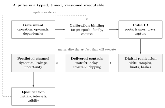
A pulse is a typed, timed, and versioned artifact. Static checks establish well-formedness; model propagation predicts controlled dynamics; experimental qualification tests the complete delivery path and feeds updated evidence back into the calibration binding.

Verification and Qualification

Static checks

Before solving any dynamics, a compiler can verify:

• every port, frame, clock, waveform, and acquisition target exists;
• units and parameter domains agree;
• durations and starts lie on supported grids;
• amplitudes, slew rates, memory, and frequency ranges satisfy hard limits;
• exclusive resources do not overlap;
• frame state is defined along every control-flow path;
• acquisition results are ready before use;
• hashes, calibration identifiers, and target versions are complete.

These checks catch malformed artifacts. They do not establish a high-fidelity gate.

Model-level checks

At model level, propagate the exact materialized samples through the declared reconstruction and transfer model, not an earlier analytic envelope. Compare the resulting unitary or channel with the target using a stated metric. For a trace-preserving channel on dimension $d$, average gate fidelity and entanglement fidelity satisfy

$$F_{\mathrm{avg}}(\mathcal E,U) = \frac{ d F_e(U^\dagger\circ\mathcal E)+1 }{d+1}.$$

Average fidelity does not by itself bound worst-case coherent error tightly, and it can hide leakage if the evaluation first projects and renormalizes. Useful checks include:

• projected and full-space evolution;
• leakage and return probabilities;
• sensitivity to uncertain parameters and timing skew;
• simultaneous-operation and spectator contexts;
• open-system propagation;
• comparison across model truncations and time steps;
• residuals against held-out calibration experiments.

Experimental qualification

An experimental ladder can include tune-up scans, Hamiltonian identification, repeated-error amplification, randomized or cycle benchmarking, leakage measurements, simultaneous-context tests, and task-representative circuits. Each answers a different question. A good fit to the same data used for tuning is not held-out validation.

Qualification should attach a validity interval and invalidation triggers: changed frequencies, gains, mixer corrections, transfer functions, neighboring calibrations, firmware, temperature, optical alignment, or device health. A pulse that was excellent last week can be the wrong executable today.

Pulse certificate

A compact certificate $\Gamma$ should record at least:

1. source operation, parameters, physical operands, and semantic convention;
2. target profile, firmware, clock domains, and calibration epoch;
3. port, frame, carrier, phase, sign, and unit conventions;
4. analytic waveform parameters and dispatched sample hashes;
5. reconstruction, modulation, predistortion, and delay models;
6. start times, durations, alignment decisions, and reserved resources;
7. Hamiltonian, dissipative, truncation, and uncertainty models;
8. predicted fidelity, leakage, sensitivity, and constraint margins;
9. experimental protocols, estimates, intervals, and held-out results;
10. expiration policy, invalidation dependencies, and provenance chain.

The certificate does not make the model true. It makes the claim inspectable and rerunnable.

Worked Lowering Example

Consider a target $X_{\pi/2}$ rotation under the resonant effective model

$$\frac{H_{\mathrm{eff}}}{\hbar} = \frac{\Omega}{2}\sigma_x$$

for a duration $T=20\,\mathrm{ns}$. A constant-envelope arithmetic model gives

$$\Omega T = \frac{\pi}{2},$$

so

$$\frac{\Omega}{2\pi} = \frac{1}{4T} = 12.5\,\mathrm{MHz}.$$

At a $2\,\mathrm{GSa/s}$ envelope rate, $\Delta t=0.5\,\mathrm{ns}$ and the duration occupies

$$N = \frac{T}{\Delta t} = 40$$

sample intervals. The pulse record still needs a port, frame, carrier, amplitude unit, reconstruction rule, start-time grid, and calibration epoch. The abrupt rectangular envelope is useful for arithmetic but usually poor as a literal command because its broad spectrum excites unwanted dynamics; an actual calibration would commonly use shaped edges or a smooth envelope.

Suppose the delivered gain is high by a fractional amount $\epsilon$. In the same simplified model, the angle error is

$$\delta\vartheta = \epsilon\frac{\pi}{2}.$$

For a unitary overrotation about the correct axis, the one-qubit average gate fidelity is

$$F_{\mathrm{avg}} = \frac{2+\cos\delta\vartheta}{3} \simeq 1-\frac{\delta\vartheta^2}{6}.$$

With $\epsilon=0.01$, this model predicts $1-F_{\mathrm{avg}}\simeq4.1\times10^{-5}$. That number is not a hardware specification. Detuning, leakage, pulse distortion, decoherence, state preparation and measurement, and repeated coherent accumulation are absent. The example shows why a control compiler must distinguish a sample-level arithmetic check from an experimentally qualified channel claim.

Common Mistakes

Treating a gate name as a waveform

$X_{\pi/2}$ identifies an intended operation, not a universal sample array. The implementation depends on physical qubit, frame, calibration, target, context, and epoch.

Omitting units and conventions

An amplitude of $0.2$ or a frequency of $5$ has no portable meaning. Record units, normalization, angular-versus-cyclic frequency, phase sign, and I/Q convention.

Assuming pulse area is always enough

Area determines angle only under a commuting resonant effective Hamiltonian. Detuning, leakage levels, time ordering, and nonlinear response make shape and context relevant.

Calling a frame update free

A virtual operation may take no waveform time, but it changes the reference state used by later controls and measurements. It must be scheduled and propagated correctly.

Simulating the analytic envelope instead of the dispatched samples

Sampling, quantization, interpolation, rounding, predistortion, and clipping can change the operation. Verify the artifact that will execute.

Inverting a transfer function without regularization

Near a transfer-function zero, exact inversion amplifies noise and control effort. Enforce bandwidth, amplitude, and robustness constraints.

Reporting projected fidelity without leakage

Projection and renormalization can discard failed population. Report leakage and in-subspace quality separately with a declared input ensemble.

Treating legal concurrency as calibrated concurrency

Nonoverlapping ports do not guarantee independent dynamics. Simultaneous Stark shifts, crosstalk, shared hardware, heating, and spectator states require contextual evidence.

Keeping no pulse provenance

Without calibration epoch, target version, sample hash, and validation record, a result cannot establish which physical operation was executed.

Exercises

1. Pulse area and frequency units

A resonant effective Hamiltonian is $H/\hbar=\Omega\sigma_x/2$. Find the constant $\Omega/(2\pi)$ needed for an $X_\pi$ gate in $40\,\mathrm{ns}$. Explain the error made by entering that number as an angular frequency in radians per second.

Solution

The area condition is

$$\Omega T=\pi.$$

Therefore

$$\frac{\Omega}{2\pi} = \frac{1}{2T} = 12.5\,\mathrm{MHz}.$$

The angular frequency is

$$\Omega = 2\pi\times12.5\,\mathrm{MHz}.$$

Entering $12.5\times10^6$ as though it were $\Omega$ under-rotates by a factor of $2\pi$. The numerical field must be typed as cyclic frequency or angular frequency rather than inferred from context.

2. Derive the equatorial rotation axis

Using the carrier and rotating-frame conventions on this page, show that a drive proportional to $\cos(\omega_d t+\phi)$ produces the RWA axis $\cos\phi\,\sigma_x+\sin\phi\,\sigma_y$.

Solution

For $R(t)=e^{-i\omega_d t\sigma_z/2}$,

$$R^\dagger\sigma_xR = \cos(\omega_dt)\sigma_x - \sin(\omega_dt)\sigma_y.$$

Multiply by

$$\cos(\omega_dt+\phi) = \cos(\omega_dt)\cos\phi - \sin(\omega_dt)\sin\phi.$$

The terms oscillating at $2\omega_d$ average away under the RWA. The surviving products have averages $1/2$, giving

$$\frac{\Omega(t)}{2} \left( \cos\phi\,\sigma_x + \sin\phi\,\sigma_y \right).$$

Changing the rotating-frame or I/Q sign convention can change the displayed sign, which is why the convention belongs in the target profile.

3. Virtual phase propagation

A pulse program applies $R_x(\pi/2)$, then a virtual frame shift by $\lambda$, then requests another nominal $x$-axis pulse. What physical equatorial axis must the second pulse use in the convention of this page?

Solution

After the frame cursor advances by $\lambda$, a pulse called $x$ in the updated frame has laboratory phase $\lambda$ relative to the old frame. Its effective generator is

$$\cos\lambda\,\sigma_x + \sin\lambda\,\sigma_y.$$

Emitting the old phase would discard the virtual $Z$ semantics. A compiler may represent the update by changing later pulse phases, by changing a numerically controlled oscillator, or by an explicit frame instruction; those representations are equivalent only if every later control and measurement uses the same frame state.

4. Duration-grid policy

A calibrated pulse has $T=21.3\,\mathrm{ns}$, while a backend requires $\Delta t=0.5\,\mathrm{ns}$. Compare rounding to $21.5\,\mathrm{ns}$ while holding amplitude fixed with rescaling amplitude to preserve area.

Solution

The nearest supported duration is $43$ ticks, or $21.5\,\mathrm{ns}$. Holding amplitude fixed increases area by

$$\frac{21.5}{21.3}-1 \simeq 9.39\times10^{-3}.$$

To preserve area in a commuting model, multiply amplitude by

$$\frac{21.3}{21.5} \simeq 0.99070.$$

Neither operation is automatically calibration preserving. The first changes angle; the second changes amplitude-dependent shifts, leakage, and spectral response. The correct policy is to select or recalibrate a supported member of the waveform family and record the materialized parameters.

5. Two-channel classical crosstalk

At one frequency, suppose

$$\mathbf H = \begin{pmatrix} 1 & 0.08\\ 0.05 & 1 \end{pmatrix}.$$

Find the command vector that would produce the target delivered vector $(1,0)^{\mathsf T}$ in this linear model. Why is this calculation not yet a safe predistortion policy?

Solution

The inverse is

$$\mathbf H^{-1} = \frac{1}{1-0.004} \begin{pmatrix} 1 & -0.08\\ -0.05 & 1 \end{pmatrix}.$$

Thus

$$\mathbf U_{\mathrm{cmd}} = \mathbf H^{-1} \begin{pmatrix}1\\0\end{pmatrix} = \frac{1}{0.996} \begin{pmatrix}1\\-0.05\end{pmatrix} \simeq \begin{pmatrix}1.0040\\-0.0502\end{pmatrix}.$$

This is only a single-frequency, linear, perfectly known inversion. A usable policy must consider the full bandwidth, uncertainty, small singular values, amplitude limits, causality, nonlinear response, and experimental validation.

6. Leakage versus conditional fidelity

A pulse leaves probability $0.02$ outside the computational subspace. After projecting onto the computational subspace and renormalizing, the remaining state has fidelity $0.999$ with the target. Why is reporting only $0.999$ misleading?

Solution

The reported number conditions on no leakage and discards two percent of the outcomes. Without correction, a simple state-overlap contribution cannot exceed roughly

$$(1-0.02)\times0.999 = 0.97902$$

when leaked population is orthogonal to the target. More importantly, leakage can persist, return with uncontrolled phase, affect spectators, and violate the assumptions of later gates or error correction. Report the leakage probability and the conditional in-subspace metric separately.

7. Feedback readiness

An acquisition begins at $1.20\,\mu\mathrm{s}$, integrates for $400\,\mathrm{ns}$, takes $180\,\mathrm{ns}$ to classify, and takes another $120\,\mathrm{ns}$ to reach the consuming sequencer. What is the earliest legal start of a conditional pulse?

Solution

The result becomes available at

$$\begin{aligned} t_{\mathrm{ready}} &= 1.20\,\mu\mathrm{s} +0.40\,\mu\mathrm{s} +0.18\,\mu\mathrm{s} +0.12\,\mu\mathrm{s} \\ &= 1.90\,\mu\mathrm{s}. \end{aligned}$$

The pulse may need to start later if its channel has a coarser alignment grid or another resource remains occupied. Starting before $1.90\,\mu\mathrm{s}$ is not merely optimistic scheduling; the branch value is unavailable.

8. Gain error and coherent accumulation

Using the worked example, compute the small-error infidelity for a $2\%$ gain error. Why can a long sequence reveal a larger effect than this one-gate number suggests?

Solution

The angle error is

$$\delta\vartheta = 0.02\frac{\pi}{2} = 0.01\pi.$$

Therefore

$$1-F_{\mathrm{avg}} \simeq \frac{(0.01\pi)^2}{6} \simeq 1.64\times10^{-4}.$$

This is a coherent overrotation. Repetitions with aligned error axes can add angles before probabilities are formed, producing oscillation or roughly quadratic early growth rather than independent stochastic accumulation. Repeated-error amplification is therefore useful for calibration, while a single average number can obscure the mechanism.

9. Design a pulse certificate test

An optimizer returns a waveform with excellent simulated fidelity for one nominal Hamiltonian. Design a minimal qualification plan before accepting it as a calibrated gate family.

Solution

First verify the exact materialized samples: units, grids, clipping, phase state, resource conflicts, and waveform hashes. Propagate those samples through the reconstruction and transfer model using a larger Hilbert-space truncation and an open-system model. Sweep held-out detuning, gain, anharmonicity, timing, and relevant simultaneous-operation contexts; report fidelity, leakage, and constraint margins.

On hardware, perform independent tune-up diagnostics and repeated-error amplification, then estimate gate and leakage behavior with a protocol suited to the gate family. Reserve circuits or parameter settings not used by the optimizer for held-out validation, including representative neighboring and concurrent contexts. Record target and firmware versions, calibration epoch, model assumptions, estimates with intervals, dependencies, and invalidation triggers. Nominal simulated fidelity alone is insufficient.

Research Status

The control-Hamiltonian framework, rotating frames, waveform shaping, virtual phase updates, optimal-control methods, and experimental gate calibration are standard. Pulse programming systems with explicit ports, frames, calibration definitions, and timing are established but not yet represented by one universally portable abstraction. OpenPulse and Quil-T are important concrete designs; hardware capabilities and grammar details continue to evolve.

Automated calibration, differentiable pulse compilation, robust ensemble optimization, learned controllers, cross-platform pulse IRs, and joint compiler-control optimization remain active research. Report improvements against baselines under the same hardware access, calibration budget, model information, drift window, and validation protocol. A shorter pulse or better simulation objective is not automatically a better experimental gate.

Further Connections

• Circuit Intermediate Representations defines the typed values, target profiles, dependencies, and lowering records from which pulse IR descends.
• Gate Decomposition chooses exact or approximate operations in the target alphabet before physical implementation is bound.
• Error-Aware Compilation selects among calibrated gate families and schedules using dated uncertainty-qualified evidence.
• Calibration Loops estimates, validates, publishes, expires, and rolls back the calibration records bound by pulse lowering.
• Quantum Software Stack places pulse lowering between target-specific compilation, controllers, measurement records, and reproducible evidence.
• Single-Qubit Gates owns rotation matrices, phase conventions, Euler synthesis, and the logical-versus-physical gate distinction.
• Multi-Qubit Gates owns controlled, exchange, SWAP, Toffoli, and measured-parity gate semantics.
• Rabi and Ramsey Control develops the basic driven and free-precession experiments used during tune-up.
• Pulse Sequences develops Ramsey, echo, CPMG, XY, and composite-sequence logic.
• Optimal Control develops objectives, constraints, adjoints, GRAPE, Krotov, and robust optimization.
• Optimal Control for Quantum Processors compares model-based, reduced-basis, black-box, hybrid, and reinforcement-learning methods and defines their deployment evidence.
• Control, Readout, and Calibration owns the physical delivery chain, acquisition inference, tune-up primitives, and real-time feedback boundary.
• Superconducting Qubits instantiates microwave, flux, resonator, leakage, and cryogenic control contracts for one major platform.
• Rotating-Wave Approximation gives the canonical derivation and validity limits for the effective resonant drive model.

References

1. D. D’Alessandro, Introduction to Quantum Control and Dynamics, 2nd ed., CRC Press (2021), doi:10.1201/9781003051268.
2. C. P. Koch et al., “Quantum optimal control in quantum technologies: Strategic report on current status, visions and goals for research in Europe,” EPJ Quantum Technology 9, 19 (2022), doi:10.1140/epjqt/s40507-022-00138-x.
3. T. Alexander et al., “Qiskit Pulse: Programming quantum computers through the cloud with pulses,” Quantum Science and Technology 5, 044006 (2020), doi:10.1088/2058-9565/aba404.
4. A. W. Cross et al., “OpenQASM 3: A broader and deeper quantum assembly language,” ACM Transactions on Quantum Computing 3, 12 (2022), doi:10.1145/3505636.
5. OpenQASM contributors, OpenQASM Language Specification: Pulse-Level Descriptions of Gates and Measurement, current and versioned specification, official specification.
6. R. S. Smith, M. J. Curtis, and W. J. Zeng, “A practical quantum instruction set architecture,” (2016), arXiv:1608.03355; see also the current Quil specification.
7. F. Motzoi, J. M. Gambetta, P. Rebentrost, and F. K. Wilhelm, “Simple pulses for elimination of leakage in weakly nonlinear qubits,” Physical Review Letters 103, 110501 (2009), doi:10.1103/PhysRevLett.103.110501.
8. D. C. McKay, C. J. Wood, S. Sheldon, J. M. Chow, and J. M. Gambetta, “Efficient $Z$ gates for quantum computing,” Physical Review A 96, 022330 (2017), doi:10.1103/PhysRevA.96.022330.
9. S. Gustavsson et al., “Improving quantum gate fidelities by using a qubit to measure microwave pulse distortions,” Physical Review Letters 110, 040502 (2013), doi:10.1103/PhysRevLett.110.040502.
10. E. Magesan and J. M. Gambetta, “Effective Hamiltonian models of the cross-resonance gate,” Physical Review A 101, 052308 (2020), doi:10.1103/PhysRevA.101.052308.
11. S. Sheldon, E. Magesan, J. M. Chow, and J. M. Gambetta, “Procedure for systematically tuning up cross-talk in the cross-resonance gate,” Physical Review A 93, 060302(R) (2016), doi:10.1103/PhysRevA.93.060302.
12. N. Khaneja, T. Reiss, C. Kehlet, T. Schulte-Herbrüggen, and S. J. Glaser, “Optimal control of coupled spin dynamics: Design of NMR pulse sequences by gradient ascent algorithms,” Journal of Magnetic Resonance 172, 296–305 (2005), doi:10.1016/j.jmr.2004.11.004.
13. S. J. Glaser et al., “Training Schrödinger’s cat: Quantum optimal control,” European Physical Journal D 69, 279 (2015), doi:10.1140/epjd/e2015-60464-1.
14. C. Brif, R. Chakrabarti, and H. Rabitz, “Control of quantum phenomena: Past, present and future,” New Journal of Physics 12, 075008 (2010), doi:10.1088/1367-2630/12/7/075008.
15. H. Ball et al., “Software tools for quantum control: Improving quantum computer performance through noise and error suppression,” Quantum Science and Technology 6, 044011 (2021), doi:10.1088/2058-9565/abdca6.
16. M. A. Nielsen, “A simple formula for the average gate fidelity of a quantum dynamical operation,” Physics Letters A 303, 249–252 (2002), doi:10.1016/S0375-9601(02)01272-0.